Candidate scoring: learning to filter without losing good decisions
Logistic regression and boosting as optimizer filters: what they predict and how to measure the cost of excluding candidates.

Series: from data to logistics decisions
- From orders to a logistics network: an optimization and machine learning project
- MILP: turning a logistics decision into a verifiable model
- Linear relaxation: how much better could a solution become?
- Greedy and local search: build quickly, then improve deliberately
- LNS: reorganizing part of a network to escape a local optimum
- Predicting demand: from a population baseline to Poisson and boosting
- Population forecasting: trends, damping, and temporal testing
- K-means: finding municipal profiles without inventing natural categories
- Candidate scoring: learning to filter without losing good decisions
- Scenarios and SAA: deciding before demand is known
Filtering has consequences
With many candidates, solving the full network can be expensive. Scoring learns which candidates tend to receive facilities in earlier solutions and proposes a shortlist. It is screening before a detailed examination: once the right candidate is removed, the optimizer cannot recover it. The aim is therefore not merely accurate classification but preserving good networks with less computation.
The aberto label indicates that a municipality received at least one module in the training solution. It is not a universal geographic truth: it depends on costs, demand, capacity, and solution quality. Inputs include local and nearby demand, weighted distance, income, rent, and scenario features. Approximate training solutions also pass their limitations to the classifier.
Two model families, one validation approach
Logistic regression transforms a feature combination into a score between zero and one; boosting combines trees and supports more flexible interactions. The module leaves one macroregion out for each fit and produces out-of-sample scores. These numbers can rank candidates, but should not be presented as calibrated probabilities of commercial success without additional evaluation.
To use the full pipeline, first prepare territorial data, scenarios, and the solutions supplying training labels. Run the command below from the repository root with a new output directory. It runs scoring experiments; it is not an instant example and cannot run from this series’ summary CSV files alone. Before a long run, inspect --help and confirm that matrices and reference tables are available.
python -m alocacao_capacitada.network.run_scoring --help
python -m alocacao_capacitada.network.run_scoring --iterations 100 --out results/scoring_tutorial_new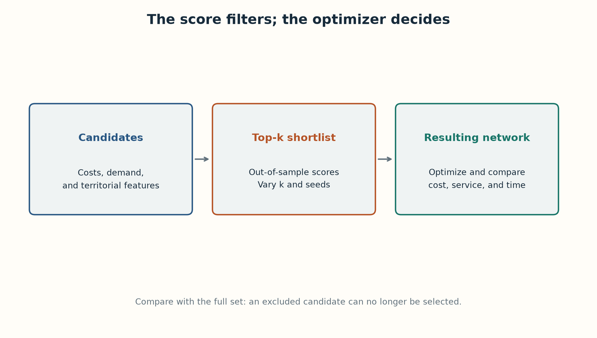
The decision is the final metric
AUC measures overall ranking, while precision@k measures the share of positives among the top k candidates. Both help, but excluding one strategic center can substantially increase network cost despite strong classification metrics. Solve the full and filtered networks under comparable budgets. Evaluate both using the same demand and transport matrix; compare cost, service, runtime, and available bounds.
excess_pct = 100 * (cost_filtered - cost_reference) / cost_referenceIf the full reference is heuristic, call the result excess cost against the reference, not distance from the optimum. A negative value can arise because the reduced problem was easier to solve within the budget; it does not prove that removing options improves the mathematical optimum. Vary k, repeat seeds, and check territorial capacity. A filter that speeds computation but prevents service to important regions has failed its purpose.