Predicting demand: from a population baseline to Poisson and boosting
How to define the target, validate geographically, and interpret errors without treating one marketplace as the whole market.

Series: from data to logistics decisions
- From orders to a logistics network: an optimization and machine learning project
- MILP: turning a logistics decision into a verifiable model
- Linear relaxation: how much better could a solution become?
- Greedy and local search: build quickly, then improve deliberately
- LNS: reorganizing part of a network to escape a local optimum
- Predicting demand: from a population baseline to Poisson and boosting
- Population forecasting: trends, damping, and temporal testing
- K-means: finding municipal profiles without inventing natural categories
- Candidate scoring: learning to filter without losing good decisions
- Scenarios and SAA: deciding before demand is known
Define what is being estimated
Observed orders reflect population, income, access, supply, and platform participation. The project learns relative purchasing propensity on Olist over a historical window. A municipality with no recorded orders may have customers served by other companies; an observed zero does not mean no market exists. Before training, define the period, geographic unit, valid orders, and handling of unmatched municipalities.
The simplest baseline allocates orders proportionally to population. A Poisson GLM lets the rate depend on features through a log link. Boosting adds trees that correct successive errors and can capture nonlinear relationships. The implementation learns orders/population with population as the sample weight, then multiplies predicted rates by population to recover order counts. This weighting should not be confused with uncontrolled row duplication.
How to apply spatial validation
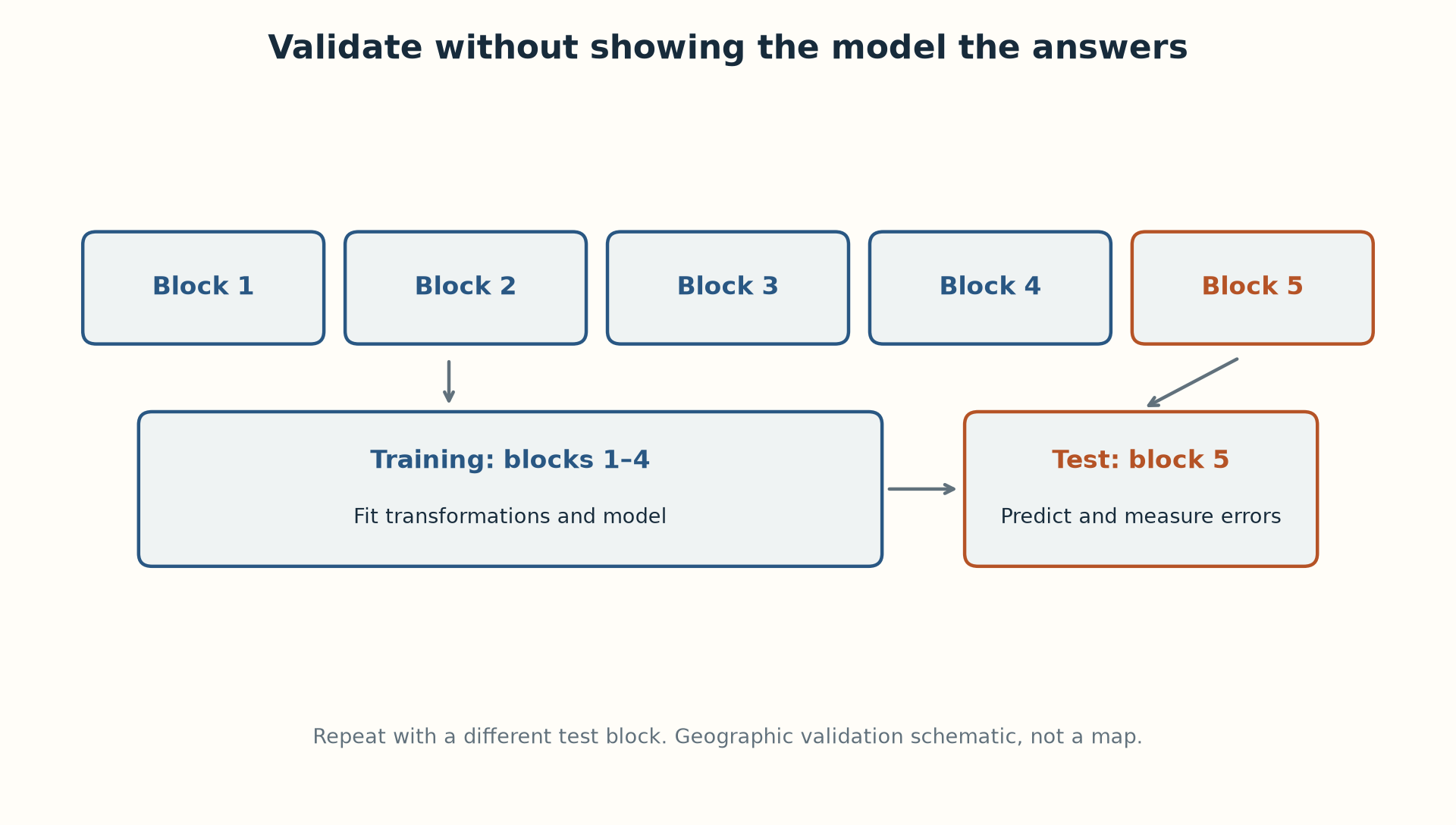
Neighboring municipalities often resemble each other. Random row splits can place very similar observations in training and test sets. The project uses five groups of states or leaves out one macroregion. Fit scaling and models only on training data, and predict each test block with a model that has not seen it. Future prediction also requires a temporal split and features available at the decision date.
from pathlib import Path
import pandas as pd
from alocacao_capacitada.ml.demand_model import cross_predict, evaluate_predictions

table = pd.read_csv(Path("results/estudo_integrado_20261001/dados_municipais.csv"))
predictions = cross_predict(table, scheme="uf")
print(evaluate_predictions(predictions).to_string(index=False))
This command runs the demand_model family; it does not exactly reproduce the integrated study’s ablation, which uses three feature sets and boosting with 150 iterations. See the linked CSV for that ablation. Keeping the same 5564 municipalities and folds lets us compare features without rewarding a model for receiving an easier sample.
| Features | Poisson deviance | Order MAE | Predicted/observed |
|---|---|---|---|
| Population only | 14.16 | 12.49 | 0.97 |
| Selected historical features | 3.98 | 6.23 | 0.95 |
| Full retrospective features | 3.14 | 5.42 | 0.91 |
Read beyond the smallest error
MAE reports average absolute error in orders. Poisson deviance measures the fit of positive predictions to counts; lower is better on the same sample. The predicted/observed ratio reveals aggregate bias: 0.91 indicates roughly 9% total underprediction even when MAE is smaller. Examine residuals by state and municipality size. High Spearman correlation indicates good relative ordering, not necessarily well-calibrated quantities.
The full ablation uses retrospective information, including information from after the order period. Its improvement does not demonstrate a forecast that would have been possible then. Even the historical subset requires publication-date checks. To decide whether the model is useful, feed its predictions into the optimizer and measure out-of-sample cost and service changes: better prediction may barely change the chosen locations.
Sources and evidence
Next: Population forecasting: trends, damping, and temporal testing