Linear relaxation: how much better could a solution become?
Learn to interpret bounds, gaps, and capacity sensitivity without mistaking a fractional solution for an operational network.

Series: from data to logistics decisions
- From orders to a logistics network: an optimization and machine learning project
- MILP: turning a logistics decision into a verifiable model
- Linear relaxation: how much better could a solution become?
- Greedy and local search: build quickly, then improve deliberately
- LNS: reorganizing part of a network to escape a local optimum
- Predicting demand: from a population baseline to Poisson and boosting
- Population forecasting: trends, damping, and temporal testing
- K-means: finding municipal profiles without inventing natural categories
- Candidate scoring: learning to filter without losing good decisions
- Scenarios and SAA: deciding before demand is known
A reference for comparison
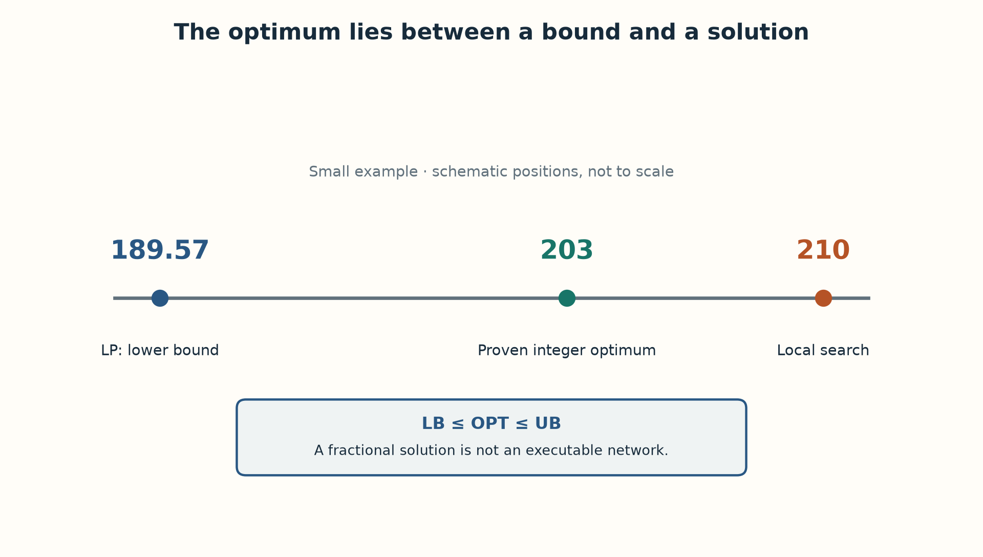
Finding a solution costing 900 does not tell us whether it is good: another might cost 500. Linear relaxation supplies a reference by allowing x and y to range between zero and one. This enlarges the feasible set, so the relaxed minimum cannot exceed the integer minimum for the same problem. Think of a budget calculation with extra permissions: if even those permissions cannot bring cost below a threshold, the original problem cannot do so either.
Opening a facility by 0.4 or splitting a region across centers may be valid in the relaxed calculation, but it does not satisfy the original binary decision. Do not round without checking assignments and capacity: rounding can create overload or raise costs. In the project, GLOP computes this reference; SCIP searches for integer decisions and can strengthen its own bound during the search.
Read the interval before the percentage
Let UB be the cost of a feasible integer solution and LB a valid lower bound. The optimum lies between them. This series uses gap = 100 × (UB − LB) / UB when UB is positive. For LNS seed 0 on 50×15, UB=885420.59 and the LP gives LB=871526.66: the gap is about 1.57%. This bounds the remaining improvement relative to that UB; it is not the probability that the solution is correct.
from alocacao_capacitada.analysis.study import tiny_instance
from alocacao_capacitada.solvers.lp_relaxation import solve_lp_relaxation
from alocacao_capacitada.solvers.milp import MilpSolver
from alocacao_capacitada.domain.evaluation import evaluate

inst = tiny_instance()
lp = solve_lp_relaxation(inst)
result = MilpSolver().solve(inst, 5.0)
ub = evaluate(inst, result.solution).total_cost
print(lp.lower_bound, ub)
print(100 * (ub - lp.lower_bound) / ub)
print(lp.y_fraction, lp.capacity_marginal_value)
The gap against the LP and the gap against the MILP bound use different references. For example, the saved 100×30 MILP run costs 1310952.57 with a bound of 1305960.58: roughly 0.38% against its own bound, whereas the comparison table reports 1.66% against the LP. Older repository results also use LB as the denominator. State the formula beside every table to avoid misleading comparisons.
How valuable is more capacity?
The capacity dual needs care: Q_i multiplies y_i in the constraint rather than appearing as a simple right-hand-side constant. The implemented local sensitivity is capacity_dual × y_fraction. It helps explore small changes to the relaxation. To decide on a real expansion, change Q_i, hold demand fixed, solve the integer model again, and compare cost, service, and expansion spending. Opening a new facility can cause a jump that a local derivative does not predict.
Sources and evidence
Next: Greedy and local search: build quickly, then improve deliberately