OptimizationPython

K-means: finding municipal profiles without inventing natural categories

Scaling, choosing k, silhouette, and stability for interpreting territorial clusters.

Jean Michael Estevez Alvarez29 Sep 2026

Clustering answers a different question

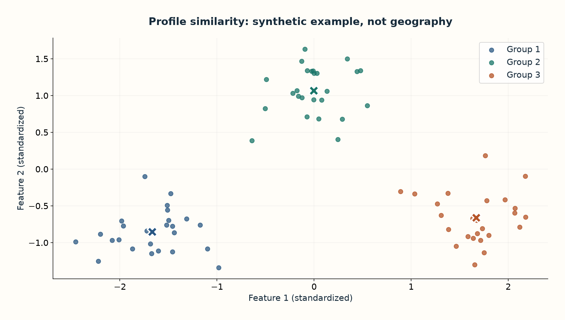
Predicting orders estimates a quantity; clustering municipalities seeks similarities. K-means organizes observations around k centroids and reduces the sum of squared distances to those centers in feature space. Here that space includes population, growth, age, income, and distance to hubs. A centroid is a numerical profile, not a recommended warehouse location.

Think of organizing a library by similarity of subject matter: categories help exploration but depend on the chosen criteria. Changing features changes what counts as close. Without scaling, a variable with large numerical values can dominate another measured as a proportion. The module applies StandardScaler and multiple initializations to reduce dependence on an unfavorable starting point.

Prepare and run

import pandas as pd
from sklearn.preprocessing import StandardScaler
from alocacao_capacitada.ml.clustering import CLUSTER_FEATURES, choose_k, fit_clusters

table = pd.read_csv("results/estudo_integrado_20261001/dados_municipais.csv")
complete = table[table["completo"]].copy()
x = StandardScaler().fit_transform(complete[CLUSTER_FEATURES])
print(choose_k(x).to_string(index=False))
labels, profile = fit_clusters(table, k=4)
print(profile.to_string(index=False))

The value k=4 demonstrates the interface; it is not a result-based recommendation. Read the candidate table first. Silhouette contrasts within-cluster closeness with separation from other clusters. The project’s stability procedure repeatedly fits on 80% subsamples, predicts labels for the full dataset, and compares partitions using adjusted Rand index. Seek interpretable groups that survive small sample changes.

From a label to a profile

Read municipality counts, median population, total population, income, and orders per group. More orders may simply reflect more people. Compare rates and dispersion as well as averages. Label numbers have no intrinsic meaning; the code reorders them by median population for readability, not as a quality ranking.

Ask whether the profiles help design scenarios or locate demand-model errors. If they merely produce attractive labels, a table by size and region may be enough. K-means favors compact groups under the chosen geometry and can obscure irregular structures or unusual municipalities. It does not establish causes: cluster membership alone does not explain why a city buys more.

Sources and evidence

• Clustering and stability
• K-means documentation

Next: Candidate scoring: learning to filter without losing good decisions

Back to the blog index