From orders to a logistics network: an optimization and machine learning project
What I built, how the algorithms connect, and what the capacitated facility location experiments demonstrate.

Series: from data to logistics decisions
- From orders to a logistics network: an optimization and machine learning project
- MILP: turning a logistics decision into a verifiable model
- Linear relaxation: how much better could a solution become?
- Greedy and local search: build quickly, then improve deliberately
- LNS: reorganizing part of a network to escape a local optimum
- Predicting demand: from a population baseline to Poisson and boosting
- Population forecasting: trends, damping, and temporal testing
- K-means: finding municipal profiles without inventing natural categories
- Candidate scoring: learning to filter without losing good decisions
- Scenarios and SAA: deciding before demand is known
The question before the algorithm
Where should distribution centers open, and which center should serve each region? Moving closer to customers reduces travel, but facilities cost money and each has limited capacity. My project turns that trade-off into a model for comparing decisions under explicit rules. This series teaches how to build and question that process, from the data to the interpretation of results.
A chain of distinct responsibilities
Data engineering preserves sources, harmonizes municipalities, and records provenance. Demand models estimate orders; population forecasts describe possible futures; clustering characterizes territorial profiles. Optimization then selects facilities and assignments. Scoring narrows the candidates, and scenario analysis checks how decisions respond to change. No stage replaces the next: predicting demand does not, by itself, determine where a facility should open.
Three scales of evidence
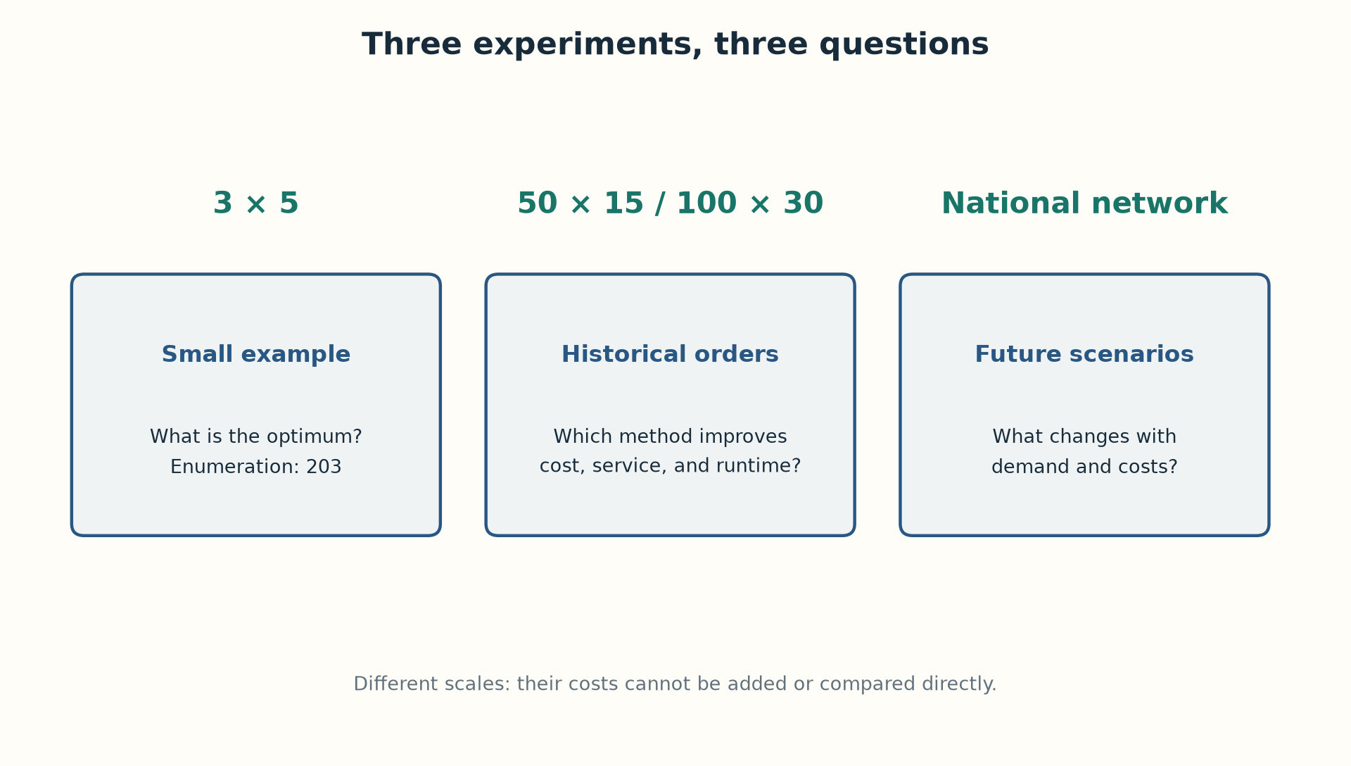
The teaching example has three centers and five regions: every decision can be enumerated, proving an optimum of 203 monetary units. The historical study uses Olist order subsets with 50 regions and 15 candidates, or 100 regions and 30 candidates. The national network adds population, propensity, and market scenarios. These experiments use different horizons and assumptions; their costs should neither be added together nor treated as directly comparable.
| Method | 50×15 cost | 100×30 cost |
|---|---|---|
| Greedy | 994102.40 | 1352149.43 |
| Local search | 920006.98 | 1339302.12 |
| MILP | 919471.41 | 1310952.57 |
| Warm-start MILP | 894531.26 | 1313883.90 |
| LNS, mean of 3 seeds | 893976.56 | 1309923.03 |
The nominal budget was ten seconds per run; fast methods finished earlier, and LNS slightly exceeded the budget in some runs. All served 100% of the selected demand, representing approximately 27.66% and 43.01% of orders in the reference universe. Mean LNS cost was 10.07% below greedy cost on 50×15, using greedy cost as the denominator. This is a computational improvement under the stated assumptions, not a measured operational saving.
How to study and reproduce
Start with the model and run the small example before changing parameters. Then compare heuristics, bounds, and seeds; only afterward add prediction and scenarios. The repository requires Python 3.12 or later and declares Cavuca as an editable dependency in the sibling ../Cavuca directory: cloning this repository alone does not guarantee a complete installation. Series examples importing alocacao_capacitada require that prepared environment. The published website contains only static pages.
The local review on 2026-10-01 ran 91 tests successfully. It also identified a census metric that differs from conventional APE and an LNS description stronger than the code actually guarantees. The articles explain both limitations. Large-experiment results quoted here were checked against existing CSV files; not all national simulations were rerun. Real investment decisions still require freight contracts, operational capacity, complete costs, and service requirements.
Sources and evidence
Next: MILP: turning a logistics decision into a verifiable model