OptimizationPython

MILP: turning a logistics decision into a verifiable model

Variables, constraints, capacity, and costs: build the three-center example and verify its optimum.

Jean Michael Estevez Alvarez23 Sep 2026

What each variable represents

Imagine a map of approved sites and regions requiring service. The model cannot invent new sites: it chooses among the supplied candidates. For each center i, y_i equals one when it opens. For each region j, x_ij equals one when center i serves it. This is a variant of the single-source capacitated facility location problem, SSCFLP. A region is an indivisible demand block in the model; this does not imply that its real orders must travel together.

The objective adds opening costs, transport costs, and penalties for unserved demand. Here f_i is fixed cost, d_j demand, c_ij transport cost per unit, and p the penalty per unserved unit. Currency and horizon must match: combining monthly rent with two years of orders distorts the decision before the solver starts.

min  sum_i f_i*y_i + sum_i,j d_j*c_ij*x_ij
     + p*sum_j d_j*(1 - sum_i x_ij)

sum_i x_ij <= 1                  (j)
sum_j d_j*x_ij <= Q_i*y_i         (i)
x_ij <= y_i                      (i,j)
x_ij, y_i in {0,1}

The first constraint allows regions to remain unserved. The second limits load, and the third links assignment to opening. A feasible solution can therefore provide insufficient service. If a contract requires full service, the first constraint must be an equality, and capacity must accommodate the indivisible blocks. A high penalty expresses an economic preference; it does not replace a contractual obligation.

A one-page laboratory

In the project environment, this program creates demands of 4, 8, 8, 4, and 2 units, three capacities of 14, and fixed costs of 33, 35, and 38. The matrix contains unit costs; the penalty is 50. An independent evaluator recomputes the solution after the solver finishes, helping detect modeling or extraction errors.

from alocacao_capacitada.analysis.study import tiny_instance, enumerate_tiny
from alocacao_capacitada.solvers.milp import MilpSolver
from alocacao_capacitada.domain.evaluation import evaluate

instance = tiny_instance()
result = MilpSolver().solve(instance, 5.0)
metrics = evaluate(instance, result.solution)
space = enumerate_tiny(instance)
print(result.status, metrics.total_cost, metrics.feasible)
print(result.solution.assignment.tolist())
print(len(space), space.custo.min())

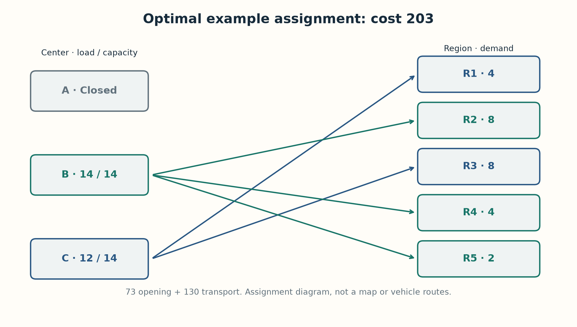
The expected result is OTIMO, cost 203, and assignment [2, 1, 2, 1, 1], using indices A=0, B=1, and C=2. B serves R2, R4, and R5, with load 14; C serves R1 and R3, with load 12. Opening cost 73 plus transport cost 130 gives 203. Including the unserved option produces 4⁵=1024 assignments; 760 respect capacity. Enumerating them and comparing costs proves this example’s optimum.

What the solver certifies

SCIP combines integer decision search, relaxations, and cuts to discard regions of the search space that cannot improve the current solution. On large instances it may stop at the time limit with a feasible solution and a different lower bound. Record both, along with service, loads, and elapsed time. Ask which constraints are missing: deadlines, shifts, inventory, and vehicle routes do not appear automatically just because a model uses MILP. An assignment map is not a delivery schedule.

Sources and evidence

• Implemented formulation
• Example and enumeration
• OR-Tools documentation

Next: Linear relaxation: how much better could a solution become?

Back to the blog index