LNS: reorganizing part of a network to escape a local optimum
Destruction, MILP repair, seeds, and convergence traces in large neighborhood search.

Series: from data to logistics decisions
- From orders to a logistics network: an optimization and machine learning project
- MILP: turning a logistics decision into a verifiable model
- Linear relaxation: how much better could a solution become?
- Greedy and local search: build quickly, then improve deliberately
- LNS: reorganizing part of a network to escape a local optimum
- Predicting demand: from a population baseline to Poisson and boosting
- Population forecasting: trends, damping, and temporal testing
- K-means: finding municipal profiles without inventing natural categories
- Candidate scoring: learning to filter without losing good decisions
- Scenarios and SAA: deciding before demand is known
Why changing one piece may not be enough
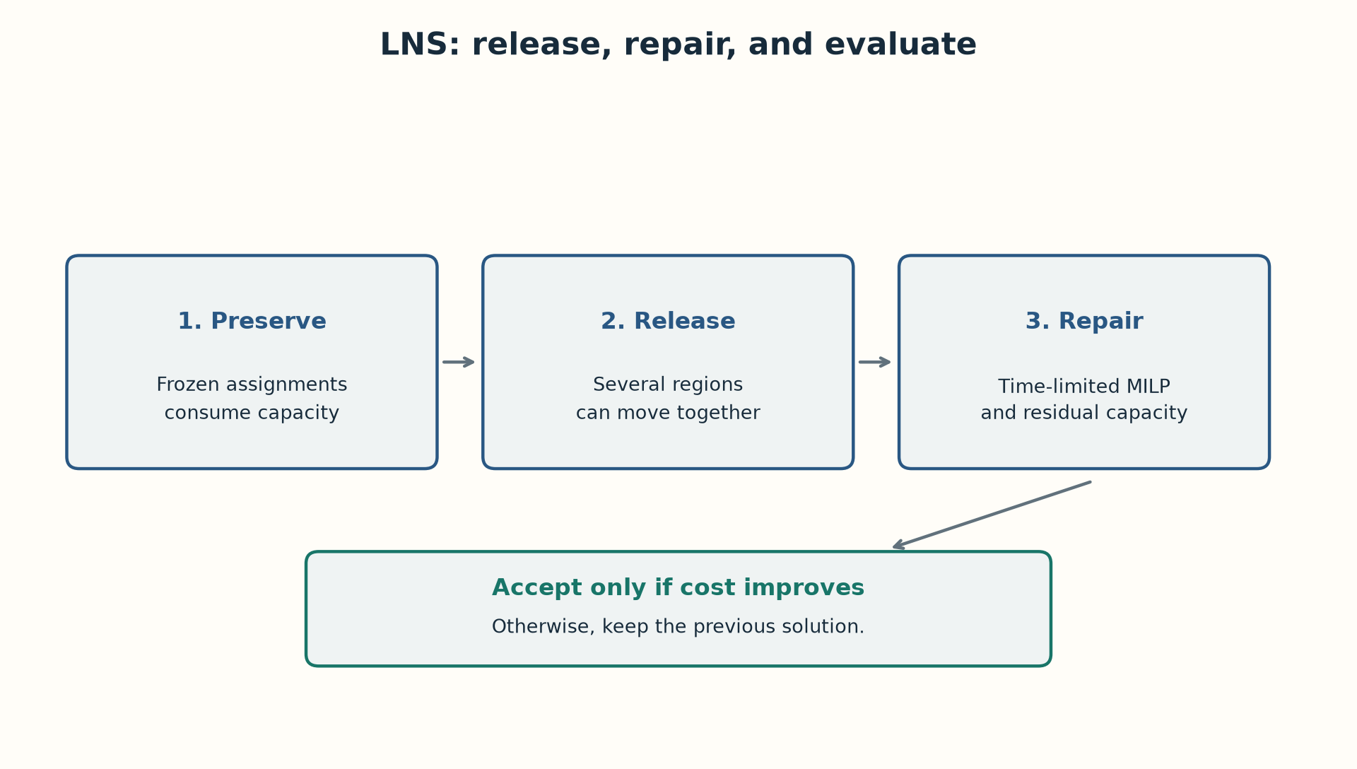
A network may need several regions to move together before a facility can close. If only small, immediately improving moves are allowed, that saving may remain unreachable. Large Neighborhood Search, or LNS, releases a set of assignments, freezes the rest, and solves how to reorganize the released portion. A useful analogy is renovating one room while keeping the rest of a house: local freedom increases without rebuilding everything.
The project alternates between selecting regions with similar cost profiles and regions associated with open centers, subject to the neighborhood size limit. MILP repair uses residual capacity: frozen demand still occupies space. A candidate is accepted only when it strictly improves cost. The incumbent cost therefore never increases, although some iterations yield no improvement.
Make a run observable
from alocacao_capacitada.analysis.study import tiny_instance
from alocacao_capacitada.solvers.greedy import NearestFeasibleGreedy
from alocacao_capacitada.solvers.lns import LnsSolver
from alocacao_capacitada.domain.evaluation import evaluate

inst = tiny_instance()
trace = []
solver = LnsSolver(NearestFeasibleGreedy(), seed=0, free_size=5,
                   sub_time_limit_s=1.0, max_iterations=10,
                   on_progress=lambda i,t,c: trace.append((i,t,c)))
result = solver.solve(inst, 5.0)
print(evaluate(inst, result.solution).total_cost)
print(trace)
The example releases up to five regions because only five exist. For larger problems, test small and medium neighborhoods under the same total budget, including initialization. Larger neighborhoods allow deeper changes but cost more time per repair; smaller ones permit more attempts. The seed controls random selection. Run multiple seeds and retain every run, not only the best one.
What a trace can tell you
A drop in the trace indicates an accepted improvement; a plateau indicates attempts without improvement. A plateau does not prove optimality. On 50×15, the three saved runs cost 885420.59, 893046.17, and 903462.92, with LP gaps of 1.57%, 2.41%, and 3.53%. Variation matters: reporting only the first would hide seed sensitivity. Three repetitions describe this sample, not a universal performance distribution.
Although the module’s opening comment describes solving the subproblem exactly, the code also accepts feasible solutions at the time limit. The precise description is budget-limited MILP repair, without guaranteed optimality for each repair. LNS also provides no global optimality certificate. Evaluate cost, service, actual runtime, and a lower bound on the same instance, and check how much improvement arrives after the first few seconds.
Sources and evidence
Next: Predicting demand: from a population baseline to Poisson and boosting