OptimizationPython

Population forecasting: trends, damping, and temporal testing

How to project population without confusing census revisions with growth or future population with guaranteed orders.

Jean Michael Estevez Alvarez28 Sep 2026

Project from an explicit baseline

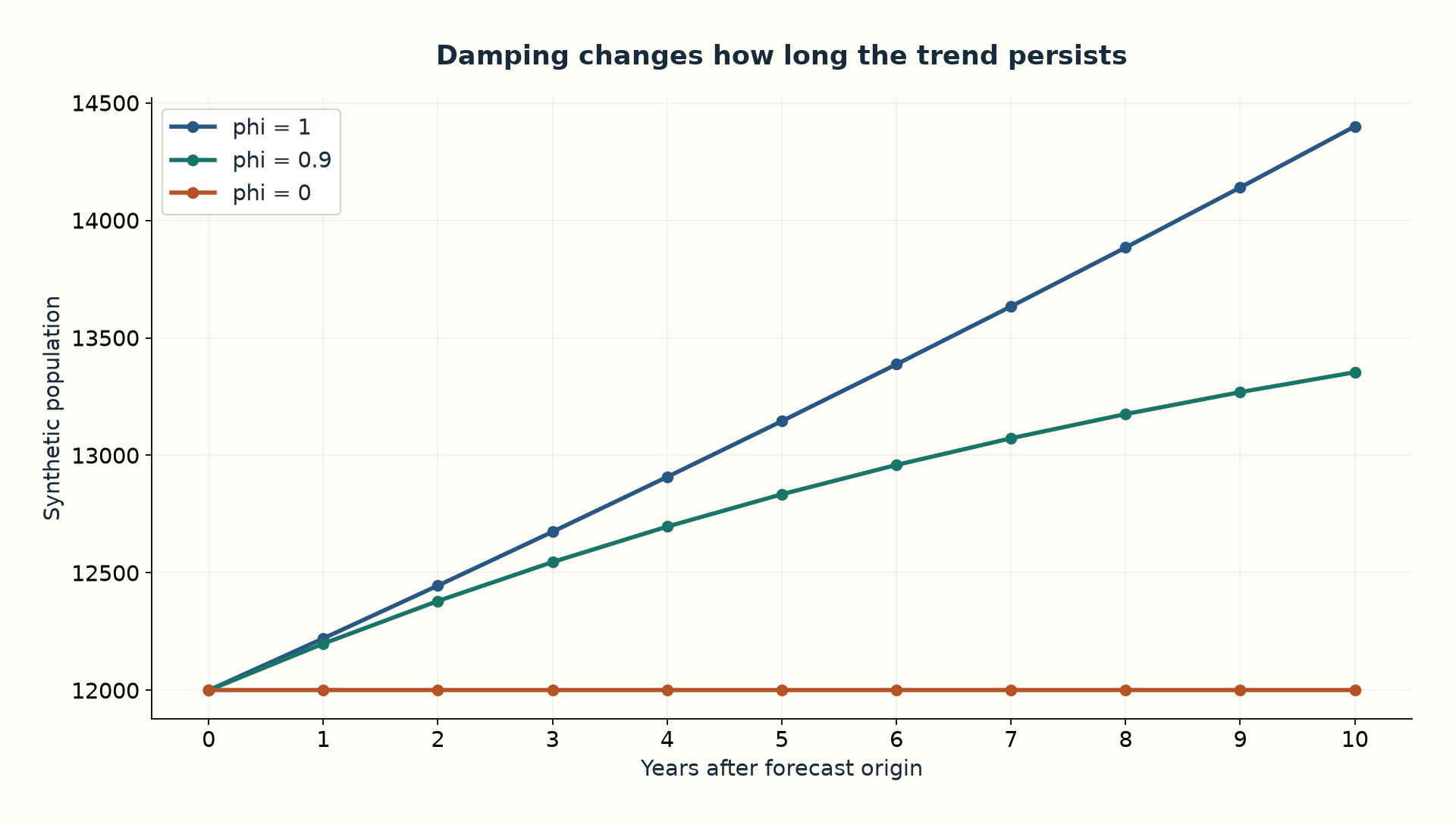
A city that grew rapidly will not necessarily keep that pace for decades. The project blends its recent growth rate with the median for municipalities in the same state and population band. Weight w controls reliance on the local trend; phi dampens its persistence. Think of considering an individual trajectory alongside a comparable group’s experience, without assuming all municipalities are identical.

g_local = (P_last / P_past)**(1 / window) - 1
g_effective = w*g_local + (1-w)*g_group
steps = sum(phi**k for k in range(1, horizon+1))
P_forecast = P_last * (1 + g_effective)**steps

With w=1, only local growth is used; with w=0, only the group reference is used. Phi=1 preserves the growth rate across the horizon; smaller values reduce its persistence. Phi=0 retains the last observed level and provides a naive baseline. Select parameters using earlier tests, rather than retrospectively choosing whichever best matches the year being predicted.

Run a controlled example

import pandas as pd
from alocacao_capacitada.ml.forecast import Config, predict

series = pd.DataFrame({2010: [10000., 20000.],
                       2020: [12000., 22000.]}, index=[1, 2])
uf = pd.Series(["SP", "SP"], index=series.index)
pred = predict(series, uf, origin=2020, horizon=5,
               config=Config(window=10, w=1.0, phi=1.0))
print(pred.round(1).to_dict())

This example uses synthetic data and should produce approximately 13145.3 and 23073.8 inhabitants. It checks the formula rather than describing real municipalities. Next, change phi and observe how the projection changes while the starting level stays fixed. Accuracy assessment requires later observations and multiple forecast origins, always comparing equivalent horizons.

What to inspect in data and metrics

IBGE estimates from before the 2022 Census and those revised afterward belong to different methodological vintages. The module separates these periods and flags interpolated years. A jump between vintages should not automatically be interpreted as real growth. Also ask whether interpolation used a value unavailable at the simulated date: temporal validation requires recreating available information, not merely sorting columns by year.

The review found that census_backtest calculates exp(|log(predicted/actual)|)−1 under an APE label. A prediction of 80 against an actual value of 100 gives 25% under that expression, while conventional APE, |predicted−actual|/actual, gives 20%. Both expressions can be studied, but they are not interchangeable. Recalculate the intended metric from predictions before quoting census percentages from the repository. That code was not changed while preparing this series.

Finally, projected population is not logistics demand. Converting it into orders requires further assumptions about propensity, market share, and purchasing frequency. Evaluate those assumptions through scenarios and test the network with fixed capacity. A more accurate forecast justifies additional complexity only if it improves the decision you actually need to make.

Sources and evidence

• Forecasting implementation and metrics

Next: K-means: finding municipal profiles without inventing natural categories

Back to the blog index