OptimizationPython

Greedy and local search: build quickly, then improve deliberately

How immediate choices, neighborhood moves, and local optima work in capacitated assignment.

Jean Michael Estevez Alvarez25 Sep 2026

The first solution need not be the last

The project’s greedy algorithm sorts regions by decreasing demand and assigns each to the lowest-unit-cost center with enough remaining capacity. Handling large blocks first aims to avoid fragmented residual capacity. It resembles placing large boxes on limited shelves first; the analogy concerns capacity, not physical dimensions, which this model does not represent.

This implementation ignores facility opening costs in its immediate choice and does not compare serving demand economically against paying the penalty. It can therefore open too many facilities. Its value is a fast initial solution and an understandable baseline. Ask whether opening costs dominate transport: if so, choosing the cheapest center per unit can be particularly shortsighted.

Improve by examining nearby alternatives

Local search starts from that solution and tries relocating a region, swapping two regions, or closing a center and reassigning its demand. It evaluates total cost changes and accepts capacity-feasible improvements. A single move may be impossible because its destination is full, while a swap releases the needed capacity simultaneously. The chosen move set therefore affects what the algorithm can find.

from alocacao_capacitada.analysis.study import tiny_instance
from alocacao_capacitada.solvers.greedy import NearestFeasibleGreedy
from alocacao_capacitada.solvers.local_search import LocalSearch
from alocacao_capacitada.domain.evaluation import evaluate

inst = tiny_instance()
for solver in [NearestFeasibleGreedy(),
               LocalSearch(NearestFeasibleGreedy())]:
    result = solver.solve(inst, 5.0)
    ev = evaluate(inst, result.solution)
    print(solver.name, ev.total_cost, ev.fixed_cost, ev.transport_cost)

Read the cost breakdown

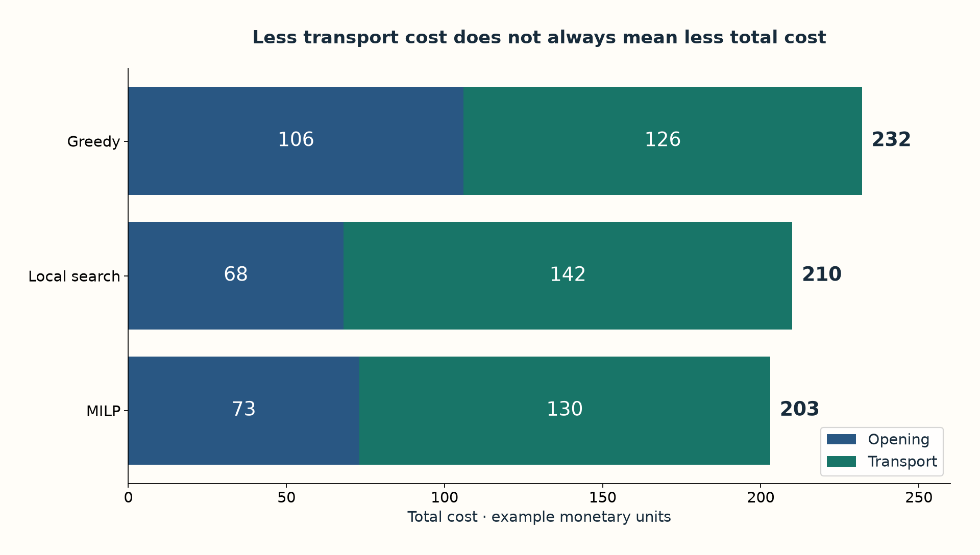
In the small example, greedy costs 232: opening 106 and transport 126. Local search reaches 210: opening 68 and transport 142. Transport becomes more expensive, but closing a facility offsets that increase. The optimum of 203 uses another combination, with opening cost 73 and transport cost 130. Looking only at distance or the number of centers would hide this trade-off.

A local optimum means no improvement was found among the examined moves after that neighborhood was fully searched. It does not prove that no better network exists. If the algorithm stops at the time limit, even neighborhood exhaustion cannot be assumed. Use these heuristics for quick responses or initialization; compare multiple instances and always retain total cost, unserved demand, and termination status.

An exercise to test your intuition

Double only the example’s fixed costs and repeat the comparison. Before running it, write down your prediction for the number of open centers. Then check whether extra transport offsets closure savings and whether unserved demand appears. The answer depends on the complete set of costs and capacities; the exercise shows why an intuitive rule needs independent evaluation.

Sources and evidence

• Greedy implementation
• Local search moves
• Example results

Next: LNS: reorganizing part of a network to escape a local optimum

Back to the blog index