Why 10,000 chunks from 20 documents are not 10,000 cases
Uncertainty in RAG, part 1: why counting chunks is not enough to tell how much information a document sample provides.

In this article
Imagine 20 documents divided into 10,000 chunks. At an 18% rate, treating them as iid Bernoulli trials gives a standard error near 0.4 percentage points and an interval of about ±0.8 points. This is an illustration, not the TAESA sample size. In the real case, the iid procedure covered fewer than a third of repetitions of 20-document samples.
The previous series on this case showed the symptom. This three-part series builds the theory that explains it and tests it on the same data. Here I answer one question: why 10,000 chunks from 20 documents are not equivalent to 10,000 independent cases. Part 2 justifies which unit the bootstrap should resample. Part 3 shows how to compute uncertainty without using the chunk as an artificial replicate.
Previous series: 33,503 chunks are not 33,503 trials
The question that defines the standard error
A standard error depends on the estimator and the mechanism by which the study is repeated. It cannot be inferred from row count alone. Here I distinguish resampling chunks from fixed documents from selecting other documents and observing all their chunks. My experiment evaluates the latter.
With documents fixed, resampling chunks within each one describes a different source of variation. Even there, unequal probabilities and local dependence matter: a single binomial formula is not sufficient. In my experiment all chunks of each selected document are observed; the uncertainty I study comes from selecting documents.
Where the randomness comes from
In the ANEEL–TAESA experiment, the search index is fixed and the outcome of each chunk was computed exactly once. Given the index, a chunk's outcome has nothing random about it: repeat the query and you get the same result. When a document enters the sample, all of its chunks enter with it, so within a document there is no sampling, only a census. The only random step in the whole procedure is the draw of which documents are evaluated.
This has a consequence that sounds paradoxical. For the 20 drawn documents, the hit rate is known without error: every one of their chunks has already been measured. For the collection, the uncertainty depends only on how much documents differ from one another. The binomial formula gets neither case right: it assigns a small uncertainty to a quantity that has none, and lends it to another whose uncertainty is much larger.
The same idea as a model
The reading above is that of finite-population sampling, which matches the validated design exactly. If you prefer a model, the intuition is the same. Suppose the outcome of chunk c in document d is made of an overall level μ, a document effect b_d and a chunk-level noise e_dc:
y_dc = μ + b_d + e_dc        Var(b_d) = σ_b²      Var(e_dc) = σ_e²

Var(ȳ) = σ_b² / K  +  σ_e² / (K · m)
This formula assumes independent documents, equal sizes, constant effect variances, and residuals independent of one another and of document effects. Under that model, increasing m reduces the second term and leaves σ_b²/K. It is an illustration; resegmenting fixed text is not equivalent to obtaining new residuals from that model.
The intraclass correlation, ρ = σ_b² / (σ_b² + σ_e²), measures how much of the total variation belongs to the document. From it come Kish's (1965) design effect and the effective sample size:
DEFF = 1 + (m − 1) · ρ

n_eff = K · m / DEFF   →   K / ρ     (m → ∞)

DEFF_Kish = 1 + ((1 + CV²) · m̄ − 1) · ρ      CV = sd(m) / m̄
In the illustrative model, with equal sizes and fixed ρ, the equivalent approaches K/ρ: about 68 for K=20 and ρ=0.293. This is not a universal bound for this corpus. Changing segmentation changes queries, outcomes and possibly correlation. With unequal sizes, ICC- and CV-based DEFF is an approximate diagnostic, not a substitute for design variance.
What the data showed
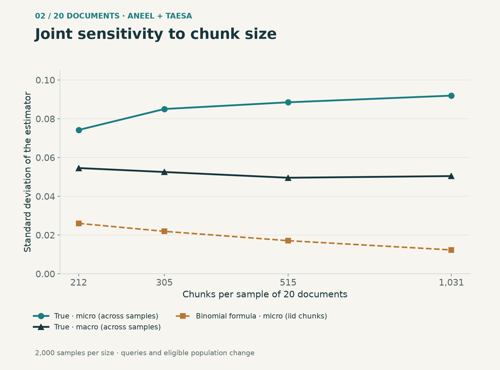
In an additional stage, I drew 2,000 samples of 20 documents using the previously computed outcomes. With 100-word chunks, the empirical micro SD was 0.0885; linearization predicts 0.0915. For macro, the values were 0.0496 and 0.0497. Against the binomial reference of 0.0171, the variance ratio is 26.8 using the empirical result and 28.7 using linearization. These are close but distinct quantities.
As a precision reference, we can divide p(1−p) by the estimated variance. With about 515 chunks per sample, the micro Bernoulli equivalent is 19.2 using empirical variance and 18.0 using linearization; the empirical macro equivalent is about 54.5. These are not additional documents or a count of independent cases.
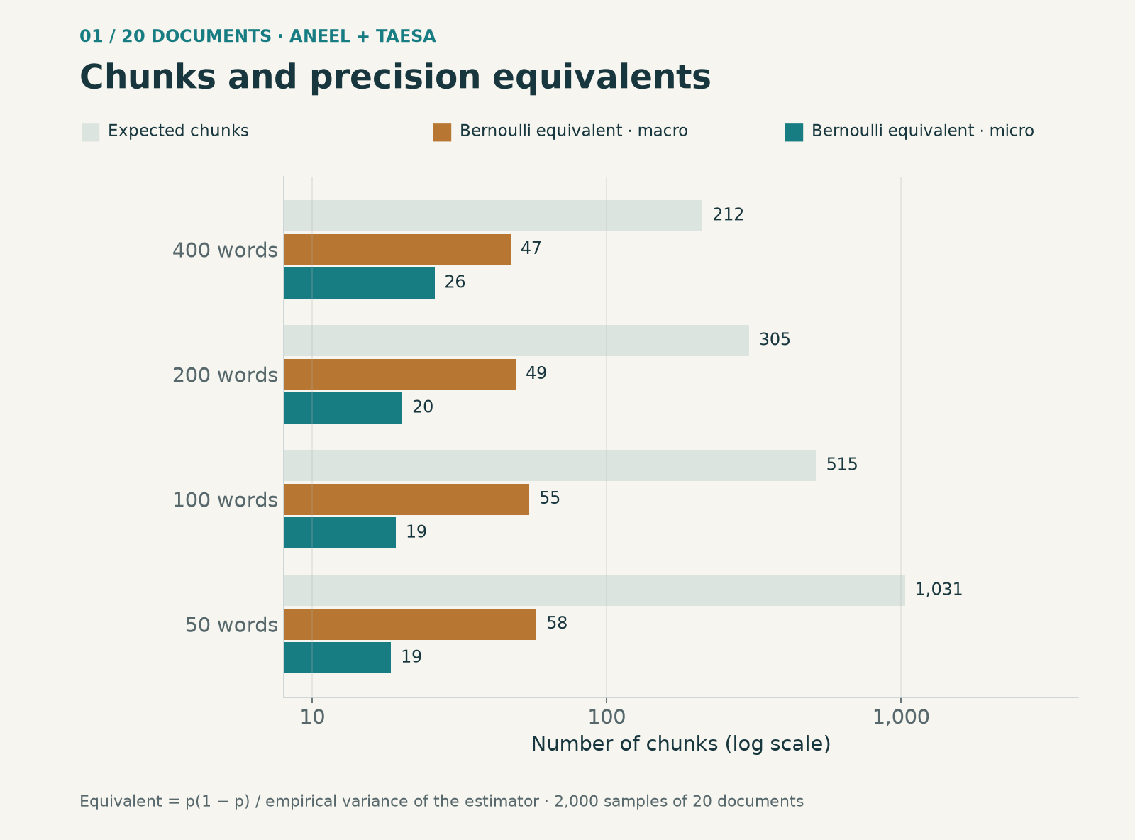
At 50 and 100 words, the same 1,300 documents remain eligible, but queries change and new samples are drawn. Expected chunks rise from 515 to 1,031; empirical micro SD changes from 0.0885 to 0.0919 and macro from 0.0496 to 0.0504. The binomial reference decreases. This describes these configurations, not a claim that every resegmentation preserves exactly the same information.
In the first version, I subtracted a binomial component from the variation between rates and interpreted the remainder as an uncertainty floor. I withdrew that interpretation: it requires conditional independence within documents, which I did not validate. For this design, the observed document rates and their variation under sampling are sufficient; no hypothetical within-document noise needs to be assigned to them.
Why chunks from one document resemble each other
Chunks from a resolution share vocabulary and structure, and a similar version from another year may compete in retrieval. These are plausible mechanisms. The ICC of 0.293 summarizes heterogeneity under the model used, but does not identify which mechanism caused each error. That attribution requires examining queries and retrieved results.
There is dependence at a smaller scale too: after removing each document's mean, neighbouring chunks still have an autocorrelation of 0.17. And at a larger scale: the document type explains 12.6% of the variation in rates. This does not undermine the argument. In the sampling view, what makes inference valid is the random draw of documents, not an assumed independence between them. If documents were drawn at random, the similarity between two versions of the same statement is part of the between-document variation that the method must reproduce.
What this argument does not say
- Chunks remain useful for measuring each document’s outcome. But resegmenting fixed text is not equivalent to collecting new independent trials and does not automatically separate noise from document difficulty.
- The binomial formula is appropriate for iid Bernoulli trials. The simulated control without heterogeneity satisfied those conditions and achieved coverage near 95%. An estimated ICC of zero alone does not establish independence or rule out local dependence.
- It does not cover every source of uncertainty. With the index fixed, the analysis measures the variation due to drawing documents. Changing the corpus composition, the retriever or the kind of question are other repetitions, with other variances.
- This does not measure final RAG quality. Hit@1 here is an attribution proxy. The reasoning extends to means of scores under a specified design and grouping, not automatically to every metric or question.
In short
The conclusion is specific: in this design, 10,000 chunks from 20 documents are not 10,000 sampling units. Documents are selected and all their chunks are observed. In TAESA, a K=20 sample contains about 515 chunks on average and a micro precision equivalent near 19.2 under the empirical reference used. The bootstrap must respect that design without promising calibration unsupported by the data.
Part 2: which unit the bootstrap should resample
Provenance and references
Data: per-chunk outcomes from the ANEEL–TAESA study (1,300 documents, 33,503 chunks of 100 words, BM25, hit@1), already presented in the previous series. The new figures come from etapa4_teoria.py, which does not recompute retrieval: it draws 2,000 samples of 20 documents from the outcomes already computed. The aggregates behind the figures and the source hashes are in the JSON file.
Download the aggregates and source hashes (JSON)
- Kish, L. (1965). Survey Sampling. Wiley.
- Cochran, W. G. (1977). Sampling Techniques (3rd ed.). Wiley.
- Miller, E. (2024). Adding Error Bars to Evals: A Statistical Approach to Language Model Evaluations. arXiv:2411.00640.
Methodological revision · October 11, 2026
I conducted the original experiments as Jean M. Estevez Alvarez. This revision distinguishes those results from subsequent checks: it preserves the original outcomes and coverage results, corrects derived quantities and adds 5,000 repetitions of the two-stage design. There was no new retrieval run, training or production evaluation.
Design revision results (JSON)
Field and Welsh (2007): models and limits of the cluster bootstrap