Computing uncertainty without artificial replicates: a document-level procedure
Uncertainty in RAG, part 3: I show the document-level calculation with formulas and code, and how I use it to compare systems and plan the sample.

In this article
In this study, document selection generates sampling uncertainty. This part explains calculations for means of grouped outcomes: hit@k, MRR or other per-query scores, when the design and grouping support them. It is not an automatic recipe for non-additive metrics, multi-document questions or stochastic judges.
Part 1: why 10,000 chunks are not 10,000 cases
Part 2: which unit the bootstrap should resample
Step 1: one row per document
For the means and clustered methods in this study, n_d, the number of observed outcomes, and s_d, their sum, are sufficient. These columns allow micro, macro and their variance approximations to be recomputed. They do not replace detailed records for auditing rankings, local dependence or temporal errors. Non-additive metrics and multi-document questions need a different specification.
If the metric is not binary, also keep the sum of squares. If the comparison is between two systems on the same queries, s_d becomes the sum of the per-query differences within the document.
Step 2: state the estimand
With unequal sizes there are two different averages, and each answers a question. The micro average, R = Σ s_d / Σ n_d, is the rate for a chunk drawn at random: what fraction of the collection's passages the system attributes correctly. The macro average, r̄, the mean of the rates s_d / n_d, is the expected rate in a typical document. In the ANEEL–TAESA collection they are 0.1846 and 0.1596. It is not a technical choice; decide it before computing and write it in the report.
If the question allows it, the macro average is easier to estimate: with 20 documents, its root mean squared error was 0.050, against 0.089 for the micro average, which depends heavily on a few large documents.
Step 3: the standard error comes from the documents
The macro average is a mean of K numbers, one per document, and its standard error is that of any mean. The micro average is a ratio, and its standard error comes from the classic linearisation of the ratio estimator: each document contributes a residual u_d = s_d − R·n_d, which measures how far its total departs from what the overall rate would give. In the formulas, se(·) is the standard error and ν the degrees of freedom.
macro   r_d = s_d / n_d      r̄ = (1/K) · Σ r_d
        se(r̄) = sd(r_d) / √K                       ν = K − 1

micro   N = Σ n_d            R = Σ s_d / N        u_d = s_d − R · n_d
  CR1   se(R) = √( K/(K−1) · Σ u_d² ) / N          ν = K − 1
  CR2   se(R) = √( Σ u_d² / (1 − n_d/N) ) / N      ν = Imbens–Kolesár

95%     θ̂ ± t(0.975; ν) · se(θ̂)
CR1 applies the K/(K−1) correction. CR2 adjusts residuals under a working model; here that model is independence. The approximate Imbens–Kolesár degrees of freedom reflect weight imbalance. With equal sizes the methods coincide; for macro they coincide with t on document rates. These are approximations, not guarantees of nominal coverage with few documents.
No step uses the number of chunks as the sample size. n_d enters only as the document's weight. That is the difference from the binomial formula, where N appears in the denominator as if each chunk were a case.
Step 4: the interval, with the degrees of freedom in plain view
Degrees of freedom describe the interval approximation, not a literal number of independent documents. With 20 documents and 764 chunks, CR2 gave ν=3.76 and a micro interval of [−0.023, 0.308]. Iid Wald gave [0.118, 0.167], missing the target of 0.185. I report K and ν separately: these are nominal intervals whose coverage must be assessed.
The code reproduces the deterministic formulas. Its bootstrap uses 9,999 replicates and seed 1; the original used 999 and a different sequence. Bounds can differ due to Monte Carlo variation. Select the sample documents first: the complete census already has a known rate.
import numpy as np
from scipy import stats

# df: one row per chunk (or query), columns doc_id and hit (0/1 or any score)
g = df.groupby("doc_id")["hit"].agg(n="size", s="sum")
n, s = g["n"].to_numpy(float), g["s"].to_numpy(float)
K, N = len(n), n.sum()
if K < 2 or np.any(n <= 0) or not np.isfinite(s).all():
    raise ValueError("Need at least two valid documents")

# micro: ratio estimator, CR2 with Imbens-Kolesar degrees of freedom
R = s.sum() / N
u = s - R * n
h = n / N
se_micro = np.sqrt(np.sum(u**2 / (1 - h))) / N
a = 1 / np.sqrt(1 - h)
M = -np.outer(a * n, a * n) / N
M[np.diag_indices(K)] += a**2 * n
df_micro = np.trace(M)**2 / np.sum(M * M)
ci_micro = R + np.array([-1, 1]) * stats.t.ppf(0.975, df_micro) * se_micro

# macro: mean of per-document rates, t with K - 1 degrees of freedom
r = s / n
se_macro = r.std(ddof=1) / np.sqrt(K)
ci_macro = r.mean() + np.array([-1, 1]) * stats.t.ppf(0.975, K - 1) * se_macro

# document bootstrap-t (macro): resample documents, studentise each replicate
rng = np.random.default_rng(1)
rb = r[rng.integers(0, K, (9999, K))]
sd = rb.std(1, ddof=1)
degenerate_fraction = np.mean(sd == 0)
if not np.any(sd > 0):
    raise ValueError("All bootstrap replicates have zero SE; interval unavailable")
tb = (rb.mean(1)[sd > 0] - r.mean()) / (sd[sd > 0] / np.sqrt(K))
lo, hi = np.quantile(tb, [0.025, 0.975])
ci_boot_t = (r.mean() - hi * se_macro, r.mean() - lo * se_macro)
For the micro average, the bootstrap-t follows the same logic: each replicate draws documents, recomputes the ratio and divides by that replicate's own CR1. Replicates in which every document has the same rate have no standard error and are discarded.
Step 5: choose the method for the situation
No method dominates in every case. The study's coverages, for nominal 95% intervals, suggest a guide:
| Situation | Evaluated approximation | Limitation or caution |
|---|---|---|
| Macro average, 20 or more documents | t with K − 1 df on the rates (93.0%) | iid Wald and chunk bootstrap (59.7%) |
| Micro average, unequal sizes | CR2 with Imbens–Kolesár df (85.7%) or bootstrap-t (88.4%) | CR1 (77.1%) and iid Wald (29.5%) |
| Five documents | CR2 (86.6% micro), stating that nominal coverage is not guaranteed | Bootstrap-t (71.1%) and percentile (75.0%) |
| Rate near 0 or 1 | Interval on the logit scale (not tested here) | Logit does not guarantee coverage; handle 0 and 1 |
| Types drawn first, then documents | Type approximation; two-stage revision: t 91.42% | The original strata comparator did not isolate one error |
Logit keeps bounds in the domain when the transformation is defined, but requires handling estimates at zero or one and does not guarantee coverage. I did not evaluate it here. Intersecting an interval with [0,1] preserves coverage for a proportion and does not improve it either. Report zeros, ones and degenerate replicates rather than hiding them behind a transformation.
Comparing two systems: differences by document
I compare retrievers on the same queries and aggregate differences by document. Pairing uses shared variation and can reduce variance: Var(A−B)=Var(A)+Var(B)−2Cov(A,B). It does not remove system-by-document interactions or change the sampling unit by itself.
In the ANEEL–TAESA collection, BM25's advantage over TF-IDF was 0.62 points for the micro average and 0.27 for the macro average, with an exact tie in 70% of documents. With differences this small, discrete and full of zeros, the document bootstraps covered between 85% and 89%. The micro-average CR2 (95.7%) and the macro-average t (97.4%) were the only ones to reach or exceed the nominal level. Before announcing that one system is better, it is worth checking the method in a simulation on your own data, as this study did.
Planning: precision is bought with documents
For planning with M=1,300 documents, I used t × S/√K × √(1−K/M). The approximation gives 76 documents for a half-width of 0.05 for macro and 220 for micro; without the finite-population correction, 80 and 264. It does not guarantee coverage or use CR2-specific degrees of freedom. Skewness and document influence also need checking.
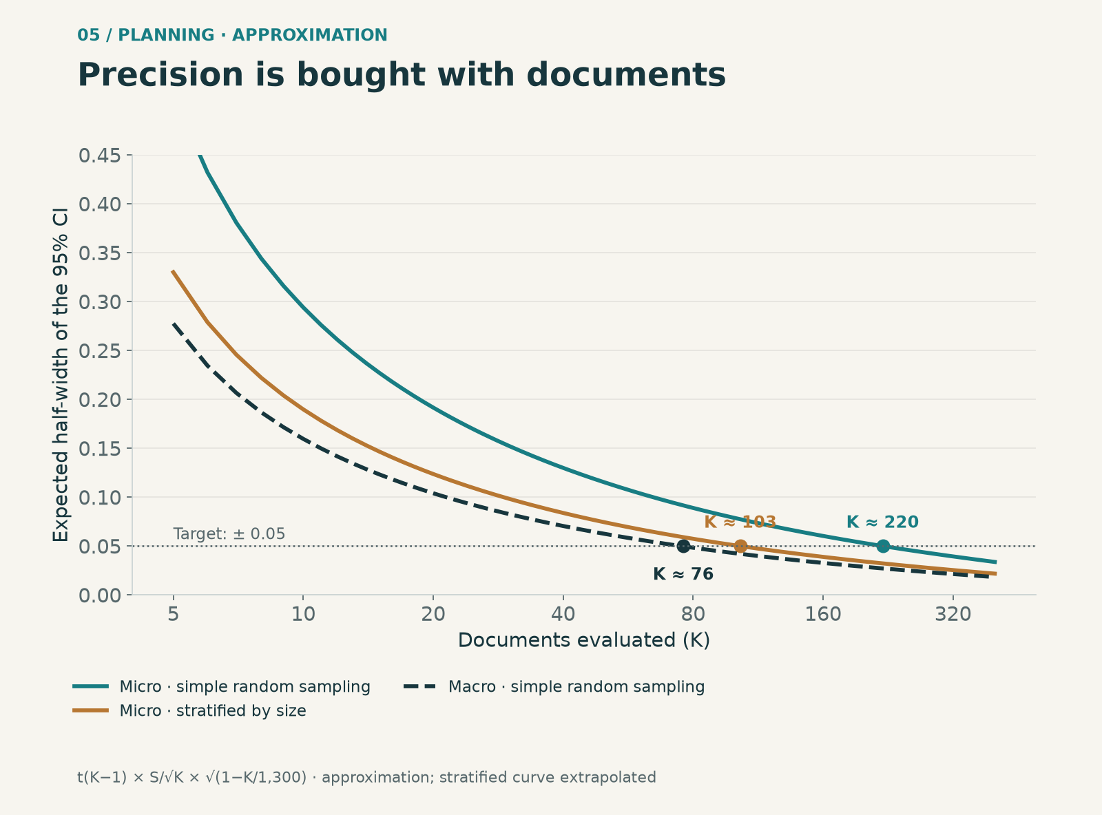
The micro average is expensive because a few large documents decide the result. The remedy lies in the design, not the calculation: stratify the draw by size. I tried separating the 129 documents with more than 76 chunks, which hold 59% of all chunks, and drawing 10 from them and 10 from the rest, with the combined ratio estimator and its stratified standard error. Consistent with part 2, the strata are fixed and documents are drawn within each one.
The standard deviation of the micro average fell from 0.092 to 0.059, and the average interval width from 0.39 with CR2 to 0.22. Coverage rose to 88.6%, still below 95%: within the stratum of small documents there is still a lot of skewness. Stratifying does not replace having more documents, but it makes each document count for more.
What to report
- The population and the design: what was drawn, at which levels and with what fraction.
- The estimand, micro or macro, and why it answers the question.
- K, N and the distribution of chunks per document.
- The interval method, the resampling unit and the effective degrees of freedom.
- The intraclass correlation and the design effect, as diagnostics rather than a substitute for the calculation.
- The fraction of documents with a rate of zero or one, and the distribution of per-document rates.
- What is left out: the fixed index, the retriever and the population of questions.
On diagnostics: the effective size N/DEFF helps explain the problem, but using it as if there were N/DEFF independent cases is another fragile approximation. In the study, that "effective-n Wald" covered 89% with 20 documents and fell to 74% with five.
Closing the series
I start with the design: what was selected, which population matters and which average answers the question. Here I aggregate by document and preserve that grouping in inference. Other designs require weights, strata, stages or questions relying on several documents. The 10,000 chunks from 20 documents illustrate the difference between measurements and sampling units; these counts alone do not determine the standard error.
Provenance and references
Method coverages and the paired comparison: ANEEL–TAESA study, with 5,000 repetitions for K = 20 and 2,000 in the sensitivity analyses. Size stratification and planning: etapa4_teoria.py, with 2,000 samples. The stratified curve in the figure extrapolates the standard deviation observed with K = 20 and is only indicative.
Download the aggregates and source hashes (JSON)
- Bell, R. M., & McCaffrey, D. F. (2002). Bias reduction in standard errors for linear regression with multi-stage samples. Survey Methodology, 28(2), 169–181.
- Imbens, G. W., & Kolesár, M. (2016). Robust standard errors in small samples: some practical advice. The Review of Economics and Statistics, 98(4), 701–712.
- Pustejovsky, J. E., & Tipton, E. (2018). Small-sample methods for cluster-robust variance estimation and hypothesis testing in fixed effects models. Journal of Business & Economic Statistics, 36(4), 672–683.
- Cochran, W. G. (1977). Sampling Techniques (3rd ed.). Wiley.
- Miller, E. (2024). Adding Error Bars to Evals: A Statistical Approach to Language Model Evaluations. arXiv:2411.00640.
Methodological revision · October 11, 2026
I conducted the original experiments as Jean M. Estevez Alvarez. This revision distinguishes those results from subsequent checks: it preserves the original outcomes and coverage results, corrects derived quantities and adds 5,000 repetitions of the two-stage design. There was no new retrieval run, training or production evaluation.
The methods in the table are evaluated approximations, not a calibrated recipe: macro t coverage of 93.0% remains below nominal 95%. The original bootstrap-t drops replicates with zero standard error and returns a point interval if all degenerate; this policy is part of the historical results and does not demonstrate certainty. In the two-stage revision, corrected variance works on average, but the t interval still covers 91.42%.
The CR1 and macro formulas shown without a finite-population correction are approximations suitable when the sampling fraction is small. For simple random sampling without replacement, macro variance includes (1−K/M); micro admits this correction in its linearization. I do not apply one global correction to multistage designs. The original references support methods under their conditions; they do not independently validate this corpus.
Design revision results (JSON)
Field and Welsh (2007): models and limits of the cluster bootstrap