What to resample: choosing the bootstrap unit in chunk-level evaluations
Uncertainty in RAG, part 2: I compare six ways to resample ANEEL and TAESA data and explain how to choose the bootstrap unit.

In this article
The bootstrap has a reputation as a method that needs no assumptions: resample, recompute, and the quantiles give you the interval. In the ANEEL–TAESA case, the chunk bootstrap contained the true value in 25% of the repetitions, worse even than the binomial formula. It did not fail for lack of replicates. It failed because it resampled the wrong unit, and no number of replicates fixes that.
In part 1 we saw that, in a chunk-level evaluation, the randomness comes from the draw of documents. Here I draw the consequence for the bootstrap: what it must resample, what each alternative captures, and what changes when there is another drawn level above the document.
Part 1: why 10,000 chunks are not 10,000 cases
The bootstrap imitates a draw
Efron’s (1979) empirical bootstrap uses the sample to approximate the estimator’s distribution. Its iid version selects the same number of units with replacement. Here the original draw is without replacement: the simple document bootstrap approximates it rather than copying it exactly. A material sampling fraction requires accounting for the finite design.
The central decision is which variation resampling should represent. Here I select documents and observe all their chunks, so the document bootstrap approximates the source of uncertainty of interest. Other designs require weights, strata and stages; automatically choosing the highest level or assuming independent selections without replacement is insufficient.
In a chunk-level evaluation, that unit is the document. Each replicate draws K document identifiers with replacement, takes all the outcomes of each drawn document and recomputes the same estimator. A document drawn twice counts twice. Nothing inside the document is touched, because nothing inside the document was drawn.
What each scheme captures
Before looking at the data, theory already says what to expect from each alternative.
- Chunks within the document. Each document keeps its size and chunks are drawn within it. The variance of the replicates is, on average, Σ n_d·p_d·(1 − p_d) / N²: internal noise only. The difference between documents, which is the real source of variation, does not appear.
- Neighboring blocks. My implementation resamples disjoint blocks within each document. It fixes the documents, not their means: resampled means change. With one block per document, within-document variation disappears. This does not evaluate every stationary-series variant in Künsch (1989).
- Documents at one level. Each replicate retains all outcomes from each selected document. This is a relevant approximation for document sampling with a small sampling fraction. Field and Welsh’s (2007) consistency results depend on the model and asymptotic regime; they do not guarantee calibration with twenty documents.
- Documents followed by chunks. This second draw adds within-document variability that is not part of the design evaluated here, where each selected document is fully observed. Increasing bootstrap variance does not guarantee exceeding actual variance or achieving conservative coverage. Field and Welsh (2007) distinguish these questions under explicit models and asymptotic regimes.
- Wild, by document. Instead of drawing documents, it multiplies each document's residual by a random weight with mean zero. It is the econometrics reference for few clusters (Cameron, Gelbach and Miller, 2008), but with very unequal sizes it can perform poorly (MacKinnon and Webb, 2017).
Six schemes put to the test
To check, I drew 2,000 samples of 20 documents from the ANEEL–TAESA collection, applied the six schemes with 999 replicates each and compared the average variance of the replicates with the true variance of the estimator across samples. If a scheme imitates the draw well, the ratio should be close to 100%.
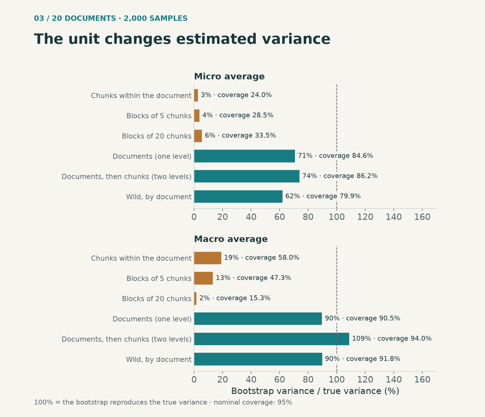
The three schemes that resample within the document captured between 3% and 6% of the true variance of the micro average and never exceeded 34% coverage. The blocks confirm the theory: moving from blocks of 5 to blocks of 20 chunks barely changes the micro average and makes the macro average worse, dropping to 15% coverage because many short documents end up with a single block. Respecting local dependence is not enough when the problem sits at the document level.
Schemes operating on documents estimated between 62% and 109% of empirical variance. With two levels, the ratio was 0.739 for micro and 1.088 for macro, with coverage of 86.25% and 93.95%. Adding a level does not guarantee a conservative interval. The unrestricted wild variant I implemented performed worse than the document bootstrap in these scenarios; this does not rule out other variants.
Why even the right scheme falls short
The document bootstrap estimated about 71% of empirical micro variance. Concentrated weight makes the ratio sensitive to the sample, but does not establish the mechanism behind each failure. I corrected an earlier explanation: with 129 documents exceeding 76 chunks among 1,300, the probability of selecting none in a sample of 20 is 12.17%, not a majority. A subset of large, easy documents would require its own definition and calculation.
That is why, with few documents, the interval method matters as well as the unit. The percentile method inherits the sample's skewness. The bootstrap-t, which divides each replicate by its own standard error, corrects part of it: in the original study it raised the micro average from 85.4% to 88.4% and the macro average from 91.5% to 97.2%, at the cost of wider intervals. With five documents, neither is reliable. The right unit is a necessary condition, not a sufficient one.
When there is a level above the document
The draw rule says more than "use the document". It says: use what was drawn. The original study tested this with a two-stage design. First, 6 of the 21 document types with at least eight documents are drawn (authorising resolutions, orders, quarterly reports, credit ratings...), then 4 documents within each type. The question becomes the average across types.
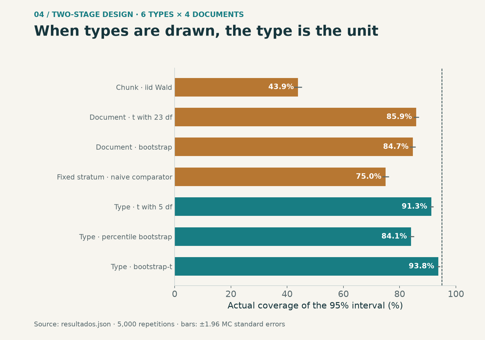
The original document methods covered about 85–86%. The “fixed strata” comparator covered 75%, but also used divisor k and normal quantiles with four documents per type: it did not isolate a single error. In the revision, I separated the conditional target for the six selected types and corrected the variance; coverage was 93.76% for that target, which differs from the mean over all types. These percentages do not answer the same question.
The simple type bootstrap is an ultimate-cluster approximation, not an exact reproduction of two-stage sampling without replacement. Both the fraction of 6 out of 21 types and the within-type draw matter. In the revision, I included variance from both stages and their finite-population corrections, checked by enumeration in a small population. Over 5,000 new repetitions, the t interval covered 91.42%: better variance estimation does not guarantee calibrated quantiles. Units, weights and stages must follow the design.
And if the documents were not drawn at random
Many evaluations use whatever documents were at hand. Then there is no draw to imitate, and the bootstrap loses its design justification. It can still be used, but resting on a model: the assumption that the documents evaluated are exchangeable with those you want to draw conclusions about. In that case, the goal of the generalisation defines the unit. If the conclusion is about other documents of the same type, the unit is the document; if it is about other types, it is the type.
That assumption must be written down in the report. No resampling fixes a biased selection: if the 20 documents were chosen because they were the cleanest, the replicates will faithfully reproduce the uncertainty of a sample of clean documents.
Four questions before resampling
- What was drawn, and in what order? The answer defines the bootstrap unit.
- Which population do you want to draw conclusions about? If there was no draw, that is what defines the unit.
- How many units are available? With few units, compare approximations and report coverage and degrees of freedom; bootstrap-t and CR2 do not guarantee nominal coverage either.
- What fraction of the population was drawn at that level? If it is large, apply a finite-population correction.
Part 3 turns all of this into a calculation procedure, with formulas, code and a way to plan how many documents to evaluate.
Part 3: computing uncertainty without artificial replicates
Provenance and references
The figures for the six schemes come from etapa4_teoria.py: 2,000 samples of 20 documents and 999 replicates per scheme; the wild bootstrap uses Webb weights and is studentised with CR1. Those for the two-stage design and the bootstrap-t come from the original study, with 5,000 repetitions. Retrieval was not rerun.
Download the aggregates and source hashes (JSON)
- Efron, B. (1979). Bootstrap methods: another look at the jackknife. The Annals of Statistics, 7(1), 1–26.
- Künsch, H. R. (1989). The jackknife and the bootstrap for general stationary observations. The Annals of Statistics, 17(3), 1217–1241.
- Davison, A. C., & Hinkley, D. V. (1997). Bootstrap Methods and their Application. Cambridge University Press.
- Field, C. A., & Welsh, A. H. (2007). Bootstrapping clustered data. Journal of the Royal Statistical Society: Series B, 69(3), 369–390.
- Cameron, A. C., Gelbach, J. B., & Miller, D. L. (2008). Bootstrap-based improvements for inference with clustered errors. The Review of Economics and Statistics, 90(3), 414–427.
- MacKinnon, J. G., & Webb, M. D. (2017). Wild bootstrap inference for wildly different cluster sizes. Journal of Applied Econometrics, 32(2), 233–254.
- Rao, J. N. K., & Wu, C. F. J. (1988). Resampling inference with complex survey data. Journal of the American Statistical Association, 83(401), 231–241.
Methodological revision · October 11, 2026
I conducted the original experiments as Jean M. Estevez Alvarez. This revision distinguishes those results from subsequent checks: it preserves the original outcomes and coverage results, corrects derived quantities and adds 5,000 repetitions of the two-stage design. There was no new retrieval run, training or production evaluation.
The methods in the table are evaluated approximations, not a calibrated recipe: macro t coverage of 93.0% remains below nominal 95%. The original bootstrap-t drops replicates with zero standard error and returns a point interval if all degenerate; this policy is part of the historical results and does not demonstrate certainty. In the two-stage revision, corrected variance works on average, but the t interval still covers 91.42%.
The CR1 and macro formulas shown without a finite-population correction are approximations suitable when the sampling fraction is small. For simple random sampling without replacement, macro variance includes (1−K/M); micro admits this correction in its linearization. I do not apply one global correction to multistage designs. The original references support methods under their conditions; they do not independently validate this corpus.
Design revision results (JSON)
Field and Welsh (2007): models and limits of the cluster bootstrap