33,503 chunks are not 33,503 trials: findings from the ANEEL–TAESA case
Part 1 of the ANEEL–TAESA case: when chunks were treated as independent tests, a nominal 95% interval covered the true value in only 29.5% of repetitions. Here I explain the experiment.

In this article
Anyone evaluating a document search system tends to follow a familiar recipe: split the texts into chunks, turn each chunk into a query and count how often the system finds the right source. Twenty documents yield a few hundred trials; the full ANEEL and TAESA collection analyzed here yields 33,503. That many trials feel like a solid measurement, with a margin of error of a few percentage points.
The question behind this article is easy to state: is that margin of error real? If I say the system is right 18% of the time, give or take three points, how far can I trust that interval?
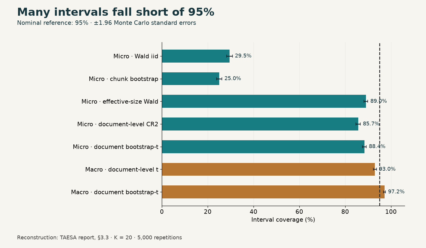
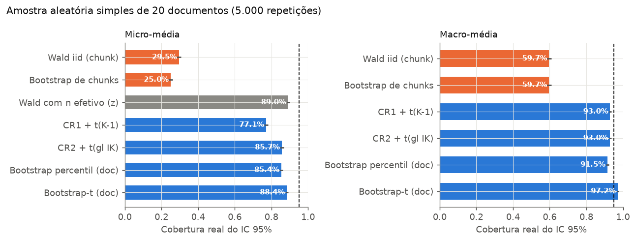
Usually there is no way to check, because the true value is unknown. In this study it is known. The outcome of all 33,503 chunks was computed once, so the hit rate of the whole collection is on record. That made it possible to repeat, 5,000 times, what an evaluator would do in practice: draw 20 documents, measure, compute a 95% interval and check whether it contains the true value. An honest 95% interval would succeed in about 95% of repetitions. The most common method, which treats each chunk as an independent trial, succeeded in 29.5%.
Put differently, seven out of ten intervals promised precision that did not exist. In this first part I describe how the test was built, why the independence assumption fails in a regulatory collection and what changes when the unit being counted becomes the document. I work from results the experiment had already computed; nothing was rerun and no production answers were evaluated. Part 2 uses these findings to discuss how to prepare and split the texts behind a regulatory RAG system.
Part 2: chunking, provisions and temporal validity
How the test was built
The collection holds 1,300 documents: 931 ANEEL acts, such as resolutions, orders and ordinances, and 369 TAESA investor relations documents, such as quarterly reports, material facts and credit ratings. This is the kind of material a company AI assistant would have to search. Some composition choices shape the result. When an act existed both as a summary and as full text, only the full text was kept. DOU texts were dropped because they repeated the official PDFs. And investor relations, which alone added up to about 14 million words, was sampled at up to 25 valid documents per type with a fixed seed. This is neither a census of the archive nor a sample of the questions its users would ask.
The task needs no human labels. Each document was split into 100-word chunks. The first 20 words of each chunk become the query, BM25 searches an index containing every other chunk, and the trial counts as a success if the top result comes from the same document. It is a cheap, objective way of asking: does the search engine recognize where this piece of text came from? Single-chunk documents were left out, because success is impossible for them: the only correct chunk is the one excluded from the search.
What 18% says, and what it does not
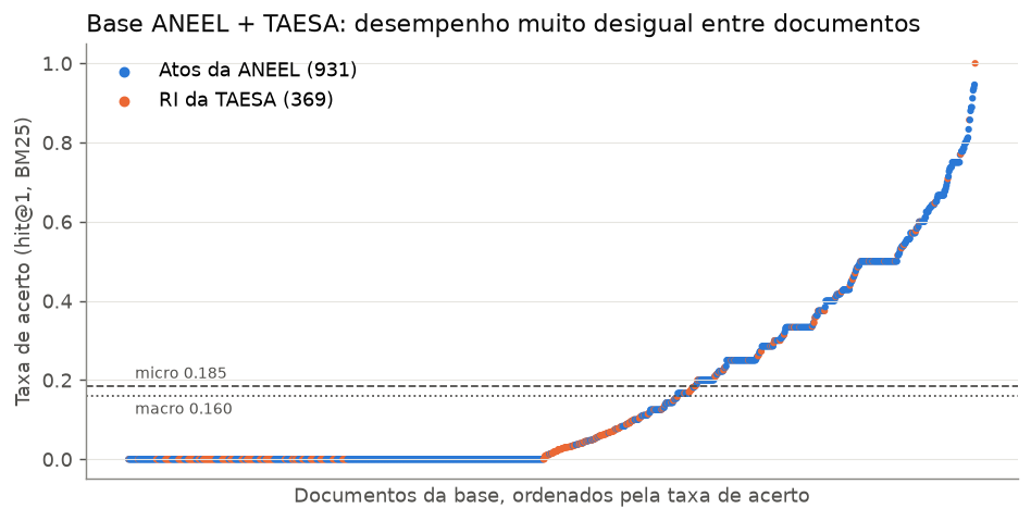
Across the whole collection, BM25 got 18.46% of queries right. That is the micro-average, where every chunk carries equal weight. Computing each document's rate first and then averaging across documents, the macro-average, brings it down to 15.96%. The 2.5-point gap appears because large documents have more chunks and therefore more votes in the micro-average. Which one to use depends on the question: the share of chunks attributed correctly, or performance on a typical document.
Results vary by type: annual regulatory accounts were near 4%, reference forms near 6%, and dividend notices at zero; normative resolutions and orders exceeded 40%. Similarity between versions is a plausible hypothesis, but the saved hit indicators do not identify the cause of each error. Testing it requires queries, rankings and review of the retrieved documents.
It is worth being precise about what this measures. Here hit@1 is a source-attribution proxy, not answer quality: it does not check expert-judged relevance, faithfulness, citations or temporal validity. An identical passage from another edition counts as an error even if it would answer a timeless question well. Documents with a zero rate are not unreachable in a RAG system; they simply were not recognized in this test. In a regulatory collection, though, mixing up 2021 and 2022 is exactly the kind of mistake that matters.
View original Figure T1: document-level distribution (in Portuguese)
The hidden assumption: every chunk is an independent trial
When a confidence interval is computed over chunks, the formula assumes each one is a fresh observation, like drawing balls from an urn. Picture a survey where you interview 20 people and ask each of them 50 similar questions. You have 1,000 answers, but answers from the same person resemble each other. The real information is closer to 20 people than to 1,000 answers.
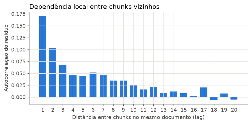
Documents behave the same way. Chunks from the same resolution share vocabulary, structure and subject; if one is easy to attribute, its neighbors usually are too. The study measured this. Intraclass correlation (ICC), which shows how much of the outcome the document explains, was 0.293, five times higher than in an earlier case with scientific papers. Even after subtracting each document's mean, neighboring chunks still have an autocorrelation of 0.17. Sizes are also very uneven: the median is seven chunks per document, but the largest 10% of documents hold 59% of all chunks.
The ICC- and size-based DEFF approximation gives 33.2 and an N/DEFF equivalent near 1,010. This is a variance reference under that model, not 1,010 documents or the sampling variance of an already observed census. Unequal sizes require the CV; the balanced formula 1+(m−1)ρ does not reproduce that value.
How to tell whether an interval is honest
This is where coverage comes in. Because the value for the whole population is known, sampling can be repeated thousands of times and the intervals containing that value can be counted. A 95% procedure should succeed in about 95% of repetitions. Coverage describes the method, not the system: it does not mean 95% of answers are correct, nor that there is a 95% probability that the value lies inside an interval already computed.
| Average | Method | Coverage | MC margin (pp) | Mean width |
|---|---|---|---|---|
| micro | Wald iid | 29.5% | ±1.3 | 0.069 |
| micro | Chunk bootstrap | 25.0% | ±1.2 | 0.057 |
| micro | Effective-size Wald | 89.0% | ±0.9 | 0.329 |
| micro | Document-level CR2 | 85.7% | ±1.0 | 0.389 |
| micro | Document-level bootstrap-t | 88.4% | ±0.9 | 0.673 |
| macro | Document-level t | 93.0% | ±0.7 | 0.206 |
| macro | Document-level bootstrap-t | 97.2% | ±0.5 | 0.243 |
The two methods that count chunks as independent, iid Wald and the chunk bootstrap, covered 29.5% and 25%. The bootstrap deserves attention because it gives the impression of being a robust method. It draws chunks with replacement; if the unit being drawn is the wrong one, repeating the draw a million times just reproduces the same error with more decimal places.
Document methods improve substantially over iid methods, but none reached 95% for micro with 20 documents: CR2 covered 85.7% and bootstrap-t 88.4%. Effective-size Wald reached 89.0%, without becoming a general solution. For macro, t covered 93.0% and bootstrap-t 97.2%. Concentrated weights and many zero rates warrant investigating sample influence; they do not by themselves establish a single cause of undercoverage.
I do not read these numbers as a universal ranking. With five documents, bootstrap-t can produce intervals wider than [0,1]. Intersecting an interval with that space preserves its coverage event for a proportion, but does not fix undercoverage. Logit can keep bounds in the domain when defined; it does not guarantee calibration either. And 3.76 CR2 degrees of freedom in one sample do not literally mean four independent documents.
Pustejovsky and Tipton (2018): cluster-robust inference with small samples
How to calculate while respecting the document
In practice the adjustment is less complicated than it sounds. For each document d, record its chunk count n_d, its hits s_d and its rate p_d = s_d / n_d. The macro-average is the mean of the rates; the micro-average is total hits divided by total chunks. With unequal sizes the two differ, so each replicate has to recompute exactly the estimator chosen.
In the document bootstrap, each replicate draws 20 document identifiers with replacement and carries along all outcomes of each one. If a document is drawn twice, its block counts twice. No new documents are created: the idea is to mimic variation across possible samples using the observed clusters. You can start with 5,000 replicates and check whether the quantiles move as that number grows. The standard error is the standard deviation of the replicate estimates, and the 95% percentile interval uses the 2.5% and 97.5% quantiles. This describes the mechanics, not a recommendation: with few clusters, that interval undercovered in this report. For the macro-average there is a direct alternative: mean rate ± t with K − 1 degrees of freedom × standard deviation of rates / square root of K. If types or families were drawn before documents, that level has to enter the calculation too.
A made-up example shows the size of the gap. Imagine 20 documents with 500 chunks each: ten never succeed and ten succeed 40% of the time. Both averages come to 0.20. Treating the 10,000 outcomes as independent gives a standard error of 0.004 and a 95% interval of roughly [0.192, 0.208]. Doing the calculation over the 20 rates gives a standard deviation of 0.2052, a standard error of 0.0459 and a t interval with 19 degrees of freedom running from about 0.104 to 0.296. The data are the same; the honest interval is more than ten times wider. These are illustrative numbers, not TAESA results.
Two caveats. First, knowing that there are 10,000 chunks and 20 documents is not enough to calculate anything; you need the outcomes, the sizes and the selection design. Second, resampling measures the uncertainty of drawing documents against a fixed index. It does not cover what would happen if the corpus were rebuilt, the retriever replaced or different questions arrived. And if the sample is a large fraction of a finite population, the corresponding correction belongs in the calculation as well.
Finer chunks make the illusion worse
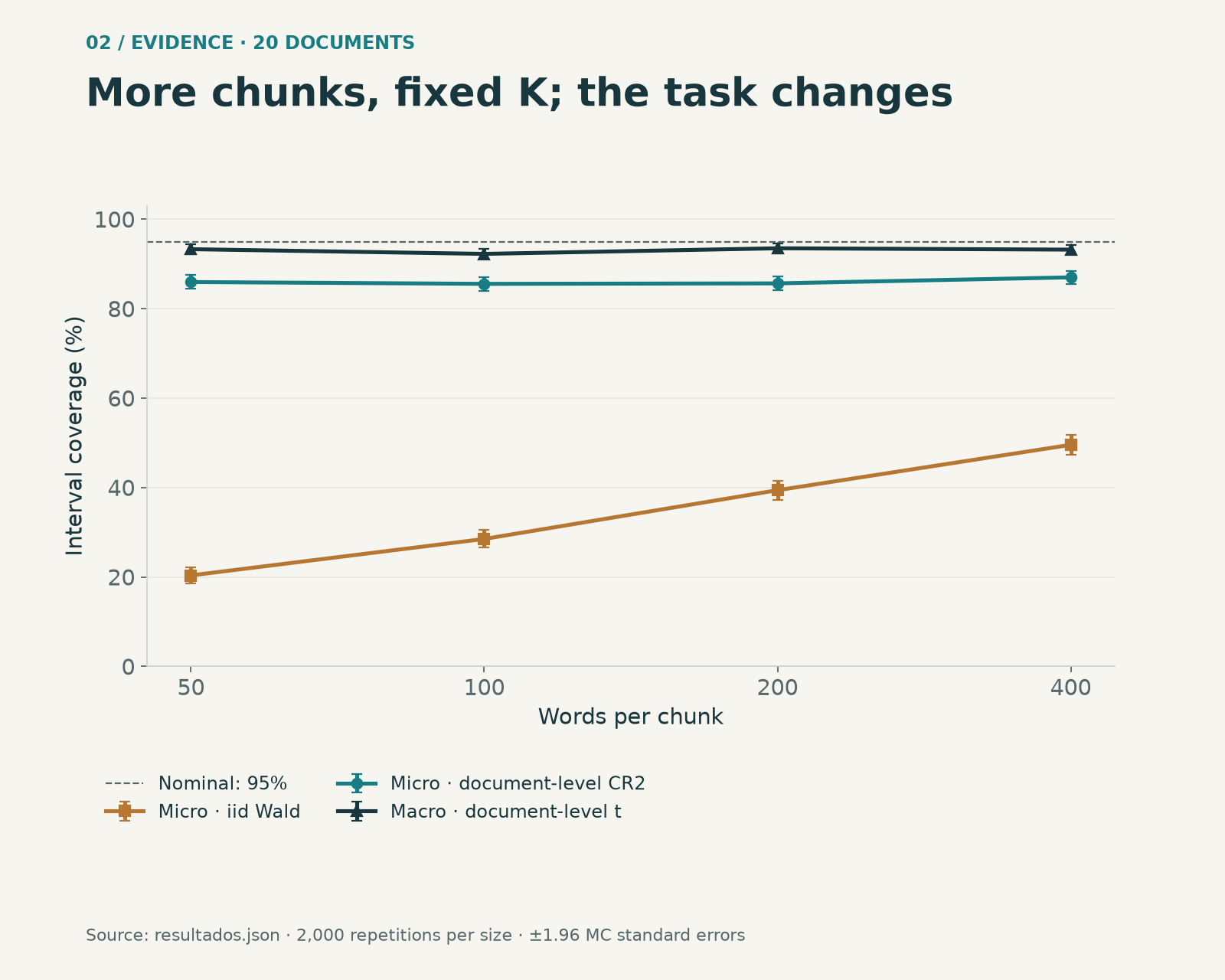
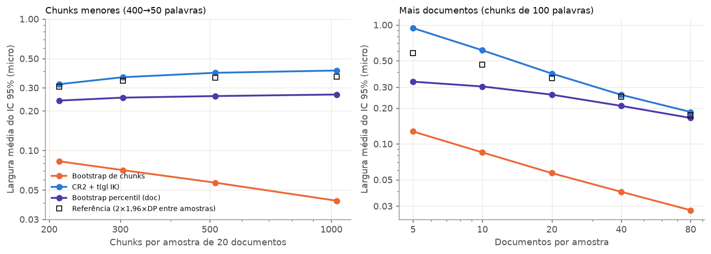
When varying chunk size, I held K=20 fixed, not the samples or queries. At 400 words, 749 documents were eligible; at 50 words, 1,300. Micro Wald coverage fell from 49.5% to 20.3%, while expected chunks per sample rose from about 212 to 1,031. This jointly varies population, queries and segmentation; it does not identify the isolated effect of finer segmentation.
More documents help, and the design decides the unit
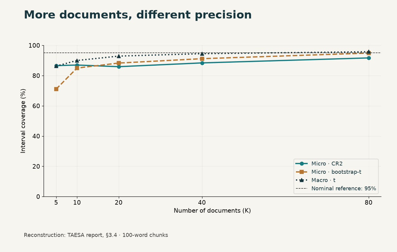
In this population, increasing K brought some methods closer to nominal: macro t covered 94.5% with 40 documents and 95.8% with 80; for micro, CR2 and bootstrap-t covered 91.7% and 94.9% with 80. These are results for specific configurations, not guarantees that a given document count suffices for any evaluation.
| K | Micro: CR2 | Micro: bootstrap-t | Macro: t |
|---|---|---|---|
| 5 | 86.6% | 71.1% | 86.3% |
| 10 | 87.0% | 85.0% | 90.0% |
| 20 | 85.9% | 88.3% | 92.9% |
| 40 | 88.4% | 91.2% | 94.5% |
| 80 | 91.7% | 94.9% | 95.8% |
I also evaluated selecting six types and four documents from each. The target is the mean across types, 0.1156. Document methods and the simple type bootstrap are different approximations; the latter does not exactly reproduce both stages without replacement. The revision added a reference with both finite-population corrections: over 5,000 new repetitions, its t interval covered 91.42%, still below nominal. The choice depends on the full design, not just thematic similarity.
What changes in a RAG decision
Back to the opening situation. Someone compares two retrievers, sees a two-point difference over thousands of trials and concludes one is better. Before accepting that, I would ask four questions. What is the population, and which estimator answers the business question? Does the comparison use the same queries, with paired differences? Does the resampling unit match what was actually drawn? And was the interval method checked, or just picked by name? In this collection, BM25's advantage over TF-IDF was 0.62 points on the micro-average, with ties in 70% of documents: a difference that small needs a well-designed evaluation to mean anything.
I would also publish the per-document distribution alongside the average. An 18% average hides that half the documents were never recognized while a minority is recognized almost every time. The study does not show that a structured legal representation would improve retrieval. It shows where to look first: at how documents are represented and how evaluation is done, before crediting any gain to the model. That is the subject of Part 2.
Continue: from chunks to regulatory provisions
Provenance, figures and limits of this reading
Source: the ANEEL–TAESA report by Jean M. Estevez Alvarez, revised on October 11, 2026, and saved results. Original figures retain the historical simulations. This revision adds a separately identified two-stage check; it does not repeat extraction or retrieval. Current and previous manifests distinguish report and aggregate versions.
Download the aggregates used in the charts (JSON)
The six original figures are provided unchanged, with Portuguese labels, as documentary material distinct from the translated illustrations. T1 shows document rates; T2, type rates; T3, simple-sampling coverage; T4, two stages; T5, width; T6, autocorrelation. Full collection texts and raw experimental files are not published.
Original Figure T1 (Portuguese)
Original Figure T2 (Portuguese)

Original Figure T3 (Portuguese)
Original Figure T4 (Portuguese)

Original Figure T5 (Portuguese)
Original Figure T6 (Portuguese)
Additional aggregates and source hashes (JSON)
Methodological revision · October 11, 2026
I conducted the original experiments as Jean M. Estevez Alvarez. This revision distinguishes those results from subsequent checks: it preserves the original outcomes and coverage results, corrects derived quantities and adds 5,000 repetitions of the two-stage design. There was no new retrieval run, training or production evaluation.
RI selection had two filters: up to 35 candidates per type after initial screening and up to 25 included after text cleaning and review. Final exclusions were not automatically replaced. Original rankings use implicit tie-breaking and do not preserve retrieved candidates; I therefore do not attribute each error to a wrong version without additional evidence.
Design revision results (JSON)
Field and Welsh (2007): models and limits of the cluster bootstrap