Why results change: capacity, data and the limits of a GNN
A mathematical reading of my experiments: how demand distributions, LP bounds and search reach help or hinder each method.

In this article
When I used a graph neural network to help choose distribution centers, the expectation seemed reasonable: if it learned to recognize good options in the training examples, the optimizer could concentrate on a smaller part of the problem. The network did learn to rank candidates with a good classification metric. Yet in the experiments, guidance based on linear programming, without prior training, led the search to better results over time. That difference between recognizing promising candidates and helping make a complete decision became the question I wanted to understand.
In the previous post, I described the AWS experimental setup and the study’s results. Here I want to examine what lay behind that comparison. A useful starting point is a concrete difficulty: a facility can look excellent on its own and still belong to a poor combination. It may be close to many customers but lack room for all of them; it may be inexpensive to open but require longer journeys; or it may compete for the same customers as another equally well-positioned facility. Optimization happens through these relationships, which give us a way to understand the algorithms’ behavior.
What changes when demand becomes concentrated
The problem I studied involves choosing which facilities to open and deciding which one will serve each customer. There is an opening cost and a service cost, and their sum should be as small as possible. That saving must respect two conditions: each customer is served by a single facility, and no facility receives demand beyond its capacity. The first condition prevents an order from being freely split across locations; the second means that one customer’s assignment changes the options available to others. Optimizing each service decision separately is therefore insufficient to organize the whole network.
To make this dependency visible, I built three small examples whose best solutions can be checked by enumerating every possible assignment. Each has three facilities with capacity for six units each, and six customers demanding two units each. Available capacity is therefore 18 and total demand is 12. I also kept opening cost at two units per facility and calculated service cost as ten times Euclidean distance times demand. Only customer positions change between panels. This lets us examine spatial distribution without confusing it with a change in capacity or in the cost rule.

In the first two scenarios, assigning each customer to its nearest facility produces loads of four units at each location. In the third, the same rule would send all twelve units to facility B, which can accommodate only six. Total capacity still exceeds demand, but some of it is in less convenient locations. To respect the limit, the solution must send some customers elsewhere and accept higher transport costs. The figure shows this redistribution: lines represent an optimal assignment, while the numbers below the panels show what would happen if we considered proximity alone.
This example gives a more precise meaning to “data distribution.” It is not just the pattern of dots on a map or average demand, but how customers compete for available alternatives. Even without geographical coordinates, an equivalent situation can arise when many customers depend on the same inexpensive connections. When opening a facility becomes expensive relative to transport, that competition gains another dimension: consolidating service saves opening costs but increases the risk of saturation and may lengthen journeys. Difficulty emerges from these characteristics together, rather than a rule that every cluster is difficult and every uniform distribution is easy.
How a mathematical simplification helps guide decisions
An optimization model lets us consider these relationships together. If yᵢ denotes the decision to open facility i and xᵢⱼ the decision to assign customer j to it, total cost can be written as z = Σᵢ fᵢyᵢ + Σᵢⱼ cᵢⱼxᵢⱼ. The first sum collects opening costs; the second collects service costs. In the original model, these decisions are either zero or one. Constraints ensure that each customer has exactly one assignment and that demand received by a facility does not exceed its capacity. Here cᵢⱼ already represents the cost of serving that customer’s entire demand through the chosen connection.
Finding the best integer combination can take considerable work. One way to obtain information before that search is to temporarily allow x and y to take values between zero and one. This version is called the linear relaxation, or LP. It can split service and consider fractional openings, possibilities that do not belong to the actual operation. Because it admits more solutions, its optimal cost cannot exceed the original problem’s optimum. It therefore gives us a lower bound: a mathematical reference for assessing how much saving might remain and which facilities appear relevant to the current instance.
The distance between that reference and an implementable solution depends on the problem’s structure. Consider three customers demanding six units each and three facilities with capacity ten, each costing one hundred to open, with no transport cost. Two facilities provide capacity twenty for demand eighteen, but cannot serve all three customers: putting two together would require twelve units at one location. We must open all three and pay three hundred. The LP, however, can distribute one third of each customer to each facility and open only 60% of each one. Each facility receives six units, has fractional capacity six, and total cost is one hundred and eighty.
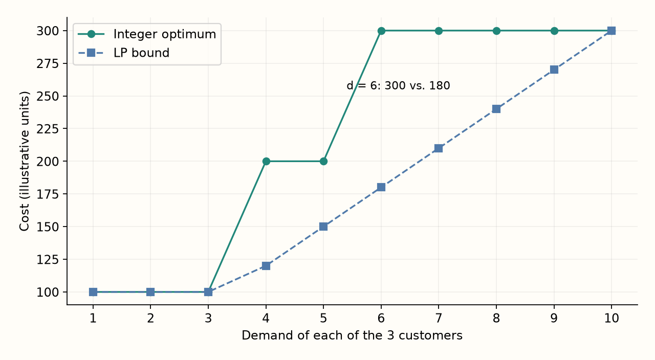
The 40% difference relative to the integer optimum is not a calculation error. It arises because the relaxation allowed decisions to be split when the original problem requires them to remain whole. The jump when demand rises from five to six marks the point where two customers no longer fit in one facility. Larger or more uneven demands can make these packing constraints especially important. Yet it would be premature to conclude that a GNN must perform better: in this example, all three facilities are symmetric and necessary. The quality of a mathematical bound and the usefulness of a candidate ranking are related, but they are not equivalent.
What the network learned and what the decision required
The GNN entered the project as another way to produce that ranking. I represented facilities and customers as graph nodes, connected through service relationships. Each node and connection carries information such as demand, capacity and relative costs. By passing messages between connected elements, the network combines that information to assign each facility a score. My model does this over three rounds. The idea was to learn which characteristics tended to identify useful facilities in previously solved problems, then use that experience to guide new ones.
To train the network, I collected solutions costing no more than 1% above the best found in each pool. A facility’s label was how often it appeared open in those solutions. The training loss, weighted binary cross-entropy, penalized disagreement between the prediction and that frequency. This is a reasonable way to learn recurrence, but it introduces an important distinction: appearing frequently in good solutions is not the same as being indispensable to a good combination in a new problem. The score ranks candidates; it does not guarantee feasibility and should not be interpreted as a calibrated probability of success.
This distinction helps explain why a favorable classification metric can coexist with an unhelpful reduction in search space. AUC, which was near 0.95 in the pilot, measures the ability to rank pairs of examples from different classes. The optimizer instead needs a set of facilities that works as a network. Excluding an important option for a difficult demand can undermine an apparently good selection. In the pilot, roughly 80% of facilities had to be retained to preserve the best-known solution in at least 80% of instances. The ranking contained learned information, but the room for safely removing options was much smaller than AUC alone might suggest.
LP guidance starts from different information, computed for the problem being solved at that moment. In the implementation, its score uses the opening value from the relaxation with a small adjustment from reduced costs. These come from the mathematical solution and, under appropriate conditions, indicate a minimum penalty associated with moving a variable away from its bound. LP therefore brings information about the current combination of capacities, demands and costs into the ranking. This provides a plausible explanation for its usefulness in the study, although it cannot attribute the entire performance difference to one cause: the learning objective, data representation and inference cost are also part of the comparison.
Why guiding search and proving a solution are different tasks
Reduced costs also allow something that a learned score alone cannot do: mathematically justify excluding certain options. Suppose the relaxation provides a lower bound of one hundred and a feasible solution already costs one hundred and twenty. For a facility whose variable is zero in the LP solution, a valid reduced cost of twenty-five means that opening it would raise the lower bound to at least one hundred and twenty-five. A solution using that facility could not improve the known solution costing one hundred and twenty. The relation is L + rᵢ ≥ U, where L is the lower bound, rᵢ is the reduced cost and U is the feasible solution’s cost.
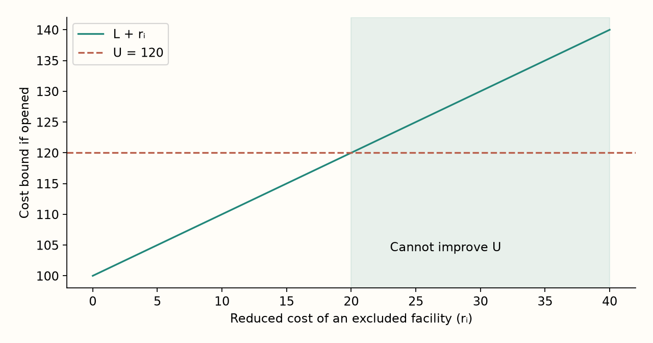
When that condition holds for every excluded facility and the restricted problem has been solved to optimality, we can certify the global result within numerical tolerances. This reasoning depends on a valid dual bound and the variable’s conditions; we cannot apply the inequality to just any number an algorithm produces. In the experiment, both LP-guided and GNN-guided expansion compute the relaxation to use its bounds. The network adds a way of ranking candidates but does not remove that computation. Its guidance therefore needed to save enough search effort to also compensate for graph preparation and inference.
This trade-off becomes clearer when we follow solutions over time. Both variants start by examining 20% of facilities, expand to 40% and 60%, and reach the full problem if necessary, with repairs to make assignments feasible. A useful ranking can make a good combination available in the early stages. If important options were excluded, the method must spend time enlarging the domain. Performance therefore depends both on which choices are made and on when they become available to the optimizer.
What the results allow us to explain
To track that evolution, I used the primal integral, a measure that accumulates deviation from a reference during execution. Finding a good solution early reduces this measure; reaching it only near the end leaves a larger deviation for longer. Across the 64 synthetic AWS instances, the mean was 0.0326 for LP expansion and 0.0712 for GNN expansion. The difference favored LP and remained significant after Holm’s statistical correction, with p = 0.00479. The final-deviation comparison had p = 0.0557 and did not pass the 5% significance threshold. The clearest evidence therefore concerns the quality of the trajectory over time, rather than final superiority established by the same criterion.
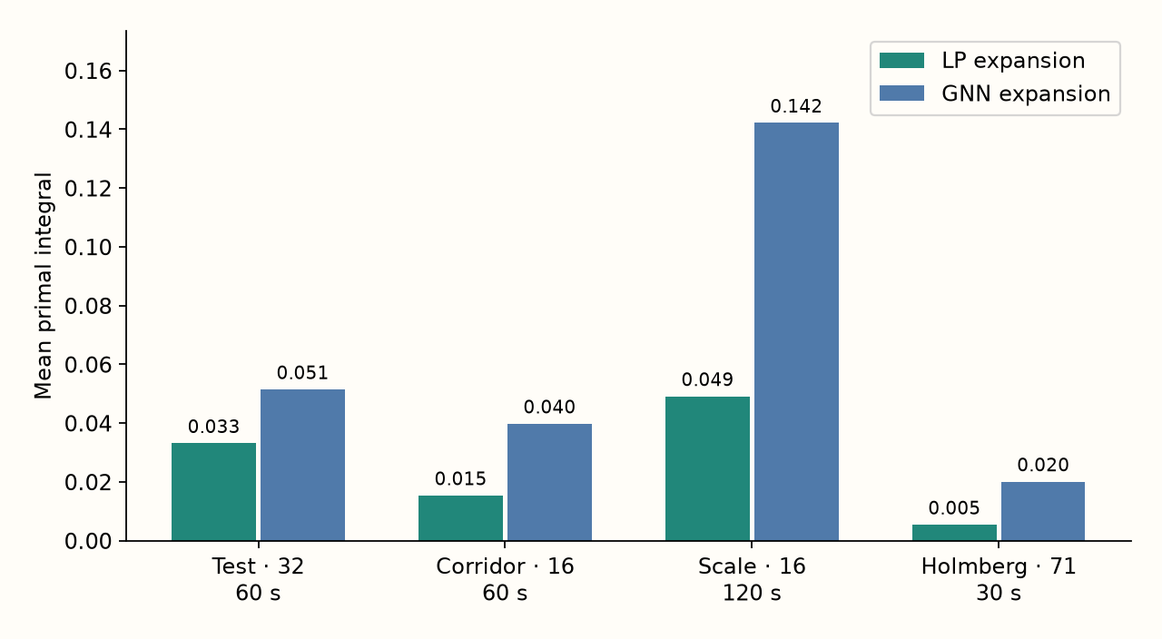
Separating results by family reveals where the distance between methods grows, but does not explain its causes on its own. The network was trained on 160 instances with 30 facilities and 150 customers in uniform and clustered geometries, and only one trained checkpoint entered optimization testing. Changing problem size, arranging customers in corridors or introducing non-Euclidean costs changes relationships encountered during training. It is plausible that this reduced the score’s usefulness, but the study did not isolate that effect from the training objective or additional computational cost. The charts show observed performance; attributing a specific share of the difference to each mechanism would require further comparisons.
There are also situations with little room for more complex guidance to help. On Holmberg, LP expansion certified 66 of 71 cases before reaching the stage containing every facility. When classical information already solves the problem quickly, learning needs to provide substantial savings to offset its additional cost. In other settings, classical guidance may weaken if many facilities receive similar evaluations or almost all must be restored to the problem. Reduction then simplifies search less, and time spent building stages may consume part of the intended advantage.
When the obstacle lies in the permitted moves
So far, we have followed how facility selection can help construct a solution. Once a feasible solution exists, another possibility opens up: keep some decisions fixed and reorganize only a group of customers. This is the principle behind the CLNS I implemented. It frees some assignments, deducts the load of fixed customers from capacity and solves a smaller problem. The benefit is to concentrate effort on a manageable change. The limitation is that the best result of this smaller problem may still be constrained by decisions that were not freed.
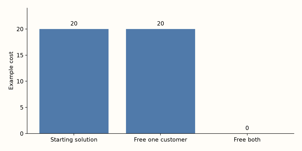
A simple example makes this limitation visible. Imagine two facilities with capacity for one unit and two customers demanding one unit each. Initially A serves customer 1 and B serves customer 2, at a cost of ten per assignment. If the customers swapped facilities, both costs would be zero. Freeing only one customer cannot make that change because its destination remains occupied by the other. Freeing both makes the swap feasible and reduces cost from twenty to zero. Available time was not the problem; the two decisions needed to be allowed to change together.
The study’s diagnostics provided evidence consistent with this limited reach. When I reran 256 subproblems with more time, 252 finished with proven optimality and no improvement. Within those permitted decisions, waiting longer did not reveal a better solution. When I increased candidate facilities per customer from ten to thirty, standalone CLNS median final deviation fell from 2.46% to 1.22%, improving 14 of 16 validation instances. The hybrid did not obtain the same benefit. Because it starts from a better solution, the remaining opportunities differ, and enlarging a neighborhood also increases the work needed to explore it.
Choosing a method by understanding the problem’s difficulty
These observations led me to view algorithm selection as a decision about which difficulty is worth tackling first. If SCIP on the full model already finds good solutions and proves their quality quickly, additional stages may offer little benefit. If the LP identifies a small set of useful facilities, expansion can use that information to reduce early work. Kernel search explores a related idea, keeping a core of candidates and adding groups ordered by reduced costs. It achieved the lowest mean integral on the synthetic test, but its comparison with LP expansion did not establish statistical superiority. The mean is therefore a clue worth investigating, rather than sufficient grounds for declaring a definitive winner.
When the difficulty lies in reorganizing an existing solution, CLNS and hybrids become attractive, provided the necessary changes fit within the freed groups. This helps interpret the results favoring the LP hybrid on larger Olist cases, although four cases are insufficient for generalization. A GNN has a plausible opportunity when many problems share a structure that training can learn and when its score is aligned with a decision that genuinely saves search. If demand-to-capacity ratios, scale or the relationship between opening and transport costs change, that advantage must be reassessed. Normalizing features helps represent the data, but does not guarantee that these changes preserve what was learned.
My study did not identify a capacitated distribution where this GNN conclusively won. To determine whether spatial concentration, demand sizes or scale changes explain a specific share of the results, one of those characteristics would need to vary while the others remained comparable. Keeping the network fixed would assess robustness; retraining it would answer the different question of how far it can adapt. This distinction prevents a convincing interpretation from becoming a conclusion that the experiments do not yet support.
What the research already supports is that problem characteristics help organize the comparison. Capacity determines which combinations are possible; the distribution of customers and costs determines which are attractive; and the search mechanism determines which will be examined within the available time. Learned guidance needs to be useful within that sequence, just as a classical rule must justify the effort it consumes. Understanding why a method works begins by following those decisions from the data to the resulting solution. That process made the findings more informative to me than a simple ranking of algorithms from best to worst.
Data and references for following the analysis
This discussion draws on my manuscript, “Learning versus classical guidance in search-space reduction for single-source capacitated facility location,” saved AWS results and project code. The chart by family uses test measurements; the others are educational examples, identified in their captions, that make the mechanisms visible. The small assignments were checked by enumeration, and the relaxation example was also verified with an LP solver. These examples add mathematical explanation to the analysis, but are not new GNN performance tests.
To place the comparison in a broader context, I also include work using GNNs for other optimization tasks. Gasse and colleagues investigate branching decisions on a graph of variables and constraints, while Qian and colleagues study uniform uncapacitated facility location. Their decisions, assumptions and formulations differ from mine, so their results need to be read in those contexts. They help explain why an unfavorable comparison in one experiment does not settle the broader discussion about learning and optimization.
Observed results by family (JSON)
Gasse et al.: learning to branch