Capacitated facility location and machine learning: models, experiments and results
An experimental analysis of where machine learning helps logistics optimization, with results, classical comparisons and limits of the evidence.

Opening a distribution center looks like a local decision: choose a place and serve its neighbors. Yet every choice changes what the rest of the network can do. In this project, I investigated whether a learned model could help decide which facilities to open and how to allocate demand, while preserving quality and counting all the time needed to produce a solution.
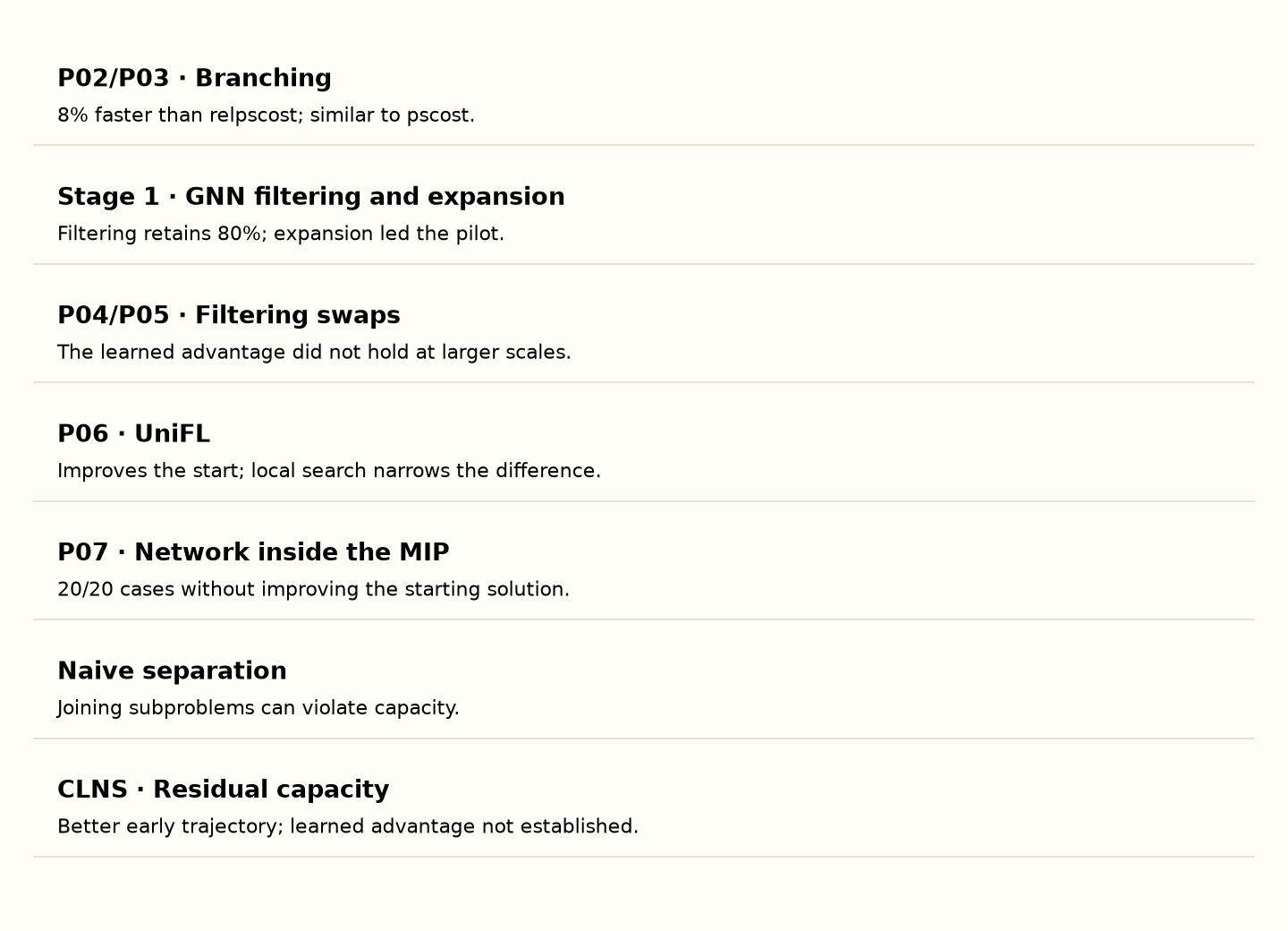
I reconstructed six research directions, P02–P07, and connected them to candidate filtering and large neighborhood search experiments. I used SCIP 10, HiGHS, OR-Tools and PyTorch on CPU. The conclusion has a specific scope: in these experiments, guiding search was more useful than replacing its decisions with predictions. A good predictive score alone did not guarantee a better logistics solution.
The problem: one demand region, one facility, limited capacity
The main model is SSCFLP: each region must be served in full by one open facility. Unlike the model with a penalty for unmet demand in the earlier series, service here is mandatory. The objective minimizes facility opening costs plus service costs, subject to each facility’s capacity.
min Σᵢ fᵢ yᵢ + Σᵢⱼ cᵢⱼ xᵢⱼ
Σᵢ xᵢⱼ = 1
Σⱼ dⱼ xᵢⱼ ≤ Qᵢ yᵢ
xᵢⱼ ≤ yᵢ
xᵢⱼ, yᵢ ∈ {0, 1}
Variable y indicates whether a facility opens; x indicates whether it serves a region. f is the opening cost, d is demand and Q is capacity. c already represents the cost of serving the region’s entire demand: multiplying it by d again would count demand twice. Costs use monetary units; demand and capacity use orders.
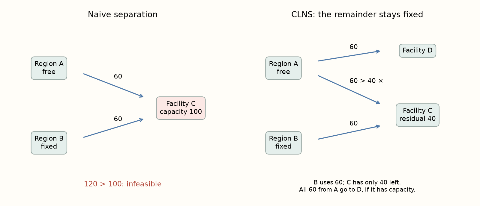
This dependence explains why splitting the map does not automatically split the problem. It is like booking seats on the same bus at two counters: each counter needs to know what the other has reserved. With 30 facilities and 150 regions, SCIP did not always prove optimality within 60 seconds; recorded certified gaps were 1.8–3.6%. In one 50 × 200 instance, the gap reached 15.6%.
Data and experimental splits
| Dataset | Instances | Purpose and reference |
|---|---|---|
| Training | 160 · 30 × 150 | Uniform and clustered; SCIP 60 s + LNS 30 s; mean gap 4.4%. |
| Validation | 32 · 30 × 150 | Seeds 1000+; parameter selection. |
| Held-out test | 32 · 30 × 150 | Seeds 2000+; prepared, not presented here as a completed final test. |
| Unseen corridor | 16 · 30 × 150 | Spatial generalization; SCIP 60 s + LNS 30 s. |
| Scale | 16 · 50 × 200 | SCIP 120 s + LNS 60 s. |
| Holmberg | 71 · 10–30 × 50–200 | Non-Euclidean costs and published optima. |
| Olist | 4 · 30 × 150 → 150 × 850 | Delivered orders by CEP3; ANTT; SCIP 300 s + LNS 120 s. |
The synthetic generator used demands U(5,35), rescaled capacities U(10,160), fixed costs proportional to the square root of capacity, and service costs of 10 × distance × demand. Uniform and clustered distributions used capacity ratios of 1.5 and 3. Instances incompatible with single-source allocation were rejected through FFD packing and a feasibility MILP.
Olist provides real orders, but that does not make every parameter an observation: opening costs and capacities are modeling assumptions. Reference gaps were 0.04%, 0.7%, 3.3% and 4.2% for 150, 300, 600 and 850 regions. These distinctions matter: beating a heuristic reference is neither proof of optimality nor evidence of savings deployed in a company.
How improvement was measured
Before comparing speed, I checked enumeration against SCIP on 13 tiny instances across three families, including tight capacities and asymmetric costs. A separate evaluator recalculated costs, single-source assignments and capacity. Timing included features, inference, linear relaxation, repair, model construction, solving and validation.

Final deviation is (U − BKS) / BKS, where U is the achieved cost and BKS is the best validated reference or published optimum. The primal integral adds the trajectory: it averages the best available solution’s deviation over the time budget, clipped to [0,1], using 1 until a solution exists. Zero means reaching the reference immediately; one means having no solution or maximum deviation throughout. Lower is better, but a lower integral does not guarantee a lower final cost.
The implementation audit found double-counted construction time, failure to carry the best solution across stages, a missing global deadline and evaluation of only one of three GNNs. The invalid timing run was archived, and the protocol was corrected with data, model and code manifests and transactional checkpoints. These timing errors did not invalidate costs or feasibility. Statistical analysis aggregates seeds by instance, uses paired comparisons, Wilcoxon tests with Holm correction and bootstrap intervals; unreached targets are censored at the budget.
Filtering candidates: a good ranking is not enough
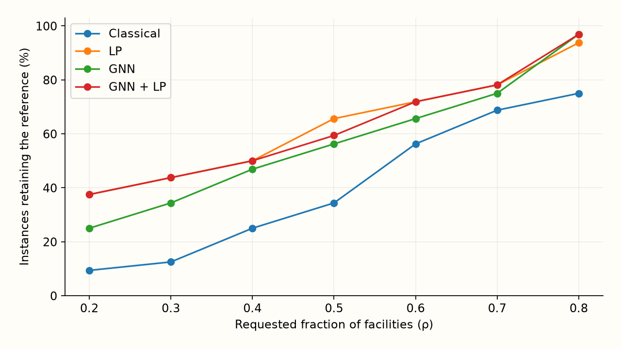
In the first stage, models ranked facilities to solve a reduced problem. The GNN achieved an AUC near 0.95, but retaining all the facilities needed by a good solution is harder than classifying individual labels correctly. On 32 validation instances, untrained linear relaxation beat the GNN from ρ = 0.2 to 0.7. At ρ = 0.8, the GNN retained the reference in 31/32 cases (96.9%), versus 30/32 (93.8%) for LP. The difference was one instance, while still keeping 80% of facilities.
UniFL: learning a starting solution, then improving it
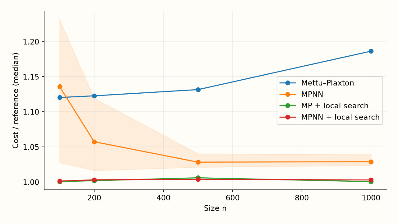
P06 studied a different variant: no capacity limits and uniform opening costs. A four-layer MPNN learned without labels by minimizing expected cost, training on n = 100 and 200. Across 56 instances, the stabilized version reached a cost ratio near 1.03 at n = 1000, compared with 1.19 for Mettu–Plaxton. At n = 1000, the reference is the best solution found, not a proven optimum. With local search, both approaches came within approximately 0.6% of their references or better: much of the advantage disappeared.
The preregistered version collapsed in three of four models: they opened a single facility and produced cost ratios between 3 and 6. The fix bounded probabilities to 0.01–0.99, clipped gradients at 1 and reduced the learning rate to 5 × 10⁻⁴. It was applied after inspecting the test and recorded as a protocol deviation; the stabilized version therefore is not an independent confirmation on untouched data.
Filtering swaps: what does speed cost?
P04/P05 reduced the swaps evaluated by local search. The learned model, trained at n = 200, achieved 3.5% deviation versus 5.1% for the classical filter without fallback. At n = 500 and 1000, that advantage disappeared. At n = 1000, the classical filter achieved roughly 47× speedup with 6.6% deviation; the learned filter, 14× with 8.8%; the random filter, 622× with 19.9%. Speedups compare paired runtimes from the same start; deviations use the best reference found.
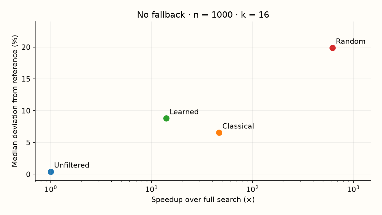
With fallback, the full neighborhood is examined again when the filter finds no improvement. Quality approaches full search, but speedup stays around 1.1–1.6×. Computing features and calling the model also takes time: the learned filter was slower than the classical one. The relevant comparison is between filters with equivalent budgets, not only against unfiltered search.
Networks inside a MIP and branching decisions
P07 embedded a Deep Sets predictor into a location-routing MIP using big-M. A MAPE of 7.5% looked favorable, but Kendall τ = 0.34 showed that ranking decisions was much harder. In 20 out of 20 cases, the neural MIP did not improve its starting solution. In one 50-customer case, the lower bound was 9222 and the cost 63746: the 591% gap uses (U − L) / L; using U as denominator gives approximately 85.5%. These conventions are not interchangeable.
| LRP method | Median deviation (%) | Mean deviation (%) | Best (%) | MIP time (s) |
|---|---|---|---|---|
| Classical continuous | 0.03 | 0.67 | 45 | 1.5 |
| NEO SCIP | 0.05 | 0.69 | 45 | 61 |
| NEO: best start | 0.08 | 1.33 | 40 | 61 |
| NEO: surrogate search | 0.30 | 1.48 | 45 | 2 |
| FLP → VRP | 4.54 | 5.60 | 15 | 0.1 |
Evaluation used OR-Tools routes on 20 CLRP instances with 20–100 customers. Best-result percentages allow ties. This is a quality comparison with separate budgets, not an equal-total-time test. The untrained classical continuous approximation tied or beat the neural alternatives.
P02/P03 learned branching decisions, reconstructed in SCIP 10 using LightGBM. On 20 instances of size 100 × 100, the learned policy was approximately 8% faster than relpscost, although it explored over three times as many nodes. It essentially tied pscost. Training used 953 samples versus roughly 100,000 in the original study; inference took 0.4% of runtime. Top-1 accuracy was 0.36 versus 0.39 for the most-fractional rule.
| Branching | Solved in 300 s | Shifted geometric time (s) | Nodes |
|---|---|---|---|
| LightGBM | 95% | 91.7 | 167 |
| pscost | 95% | 93.2 | 165 |
| relpscost | 95% | 100.1 | 49 |
| fullstrong | 90% | 107.4 | 23 |
CLNS: reorganizing one part without breaking the whole
Solving geographic clusters independently and joining them failed on three validation instances, with overloads of 690–1070 units. Repairing them left costs 19–29% above the reference. CLNS avoided this separation: it released one subproblem at a time, kept the remainder fixed, deducted its occupancy from available capacity and counted fixed costs only once.
Four neighborhoods were tested: a cluster’s interior, the border between two clusters, releasing an expensive facility and customers with the highest regret according to LP dual information. Five selectors chose which neighborhood to solve: rotation, random, ALNS, dual and learned. The LightGBM selector estimated gain per second and achieved AUC 0.76 on validation separated by instance.
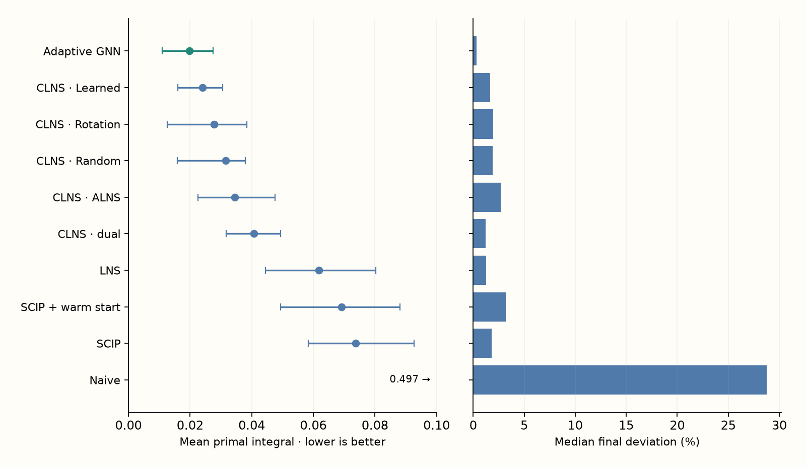
CLNS achieved mean integrals of 0.024–0.041 versus 0.062–0.074 for LNS and SCIP, with median final deviations of 1.2–2.7%. The learned selector achieved the best aggregate CLNS integral, but rotation won on roughly 62% of instances; p = 0.43 did not support statistical superiority of learning. Adaptive expansion using GNN and LP information achieved an integral of 0.0198 and median deviation of 0.32%. These are results from this validation pilot, not the reserved held-out test.
What the results establish and what they do not
The project identified useful mechanisms and concrete limits. Search preserved global feasibility when subproblems respected residual capacity. Learned models ranked candidates and neighborhoods, but did not systematically outperform equivalent classical alternatives. LP was a strong filter; Mettu–Plaxton with local search absorbed much of the neural advantage; a continuous approximation competed with the neural MIP. The relevant number depends on the decision: time to a good solution, final cost or proof of optimality.
Execution used CPU, with up to three processes on four physical cores, and mostly synthetic data. Holmberg provides an external anchor; in other cases BKS remains heuristic. These are methodological reconstructions in an open environment, not exact reproductions of historical environments or Gurobi. Changes in solver, scale and budget limit how far the conclusions transfer. This publication’s charts were rebuilt from saved CSVs; they do not represent new experimental runs.