No silver bullet in optimization: what I learned by testing a GNN on AWS
From experimental setup to results: when restricting search helps, when learning adds no benefit, and why context changes the decision.

I started with an appealing idea: train a graph neural network to recognize promising distribution center locations, then let an optimizer solve a smaller problem. The network learned to rank candidates quite well. But measuring the complete decision raised an uncomfortable question: was the improvement coming from learning, or from organizing search more effectively?
The paper behind this post answers that question through controlled comparisons, a held-out test and a repeat on AWS. The main result favored classical guidance based on linear relaxation, without training. That does not establish that GNNs are useless or that classical algorithms always win. It establishes something more specific: for this problem, trained model and computational budget, the added complexity did not deliver the expected advantage.
This continues the post about the initial experiments. In that account, the held-out test was still reserved; here it has been run in two environments. I describe the results documented in the current version of my research manuscript.
First, understand the logistics decision
The problem is to choose which facilities to open and which facility serves each region. Opening costs money, transport costs money, and each facility has limited capacity. A region must also receive all its demand from one facility: it cannot be split or left unserved. This is the single-source capacitated facility location problem, or SSCFLP.
Capacity connects decisions that look independent. If two regions each need 60 units, they cannot both fit into a facility with capacity 100. Solving each region separately can produce two reasonable answers that become impossible when combined. It is like two people booking the same seats without sharing their reservation records. A good system must coordinate decisions, not just make good isolated recommendations.
What I built to investigate the question
I built an experimental framework with instance generators, separate training, validation and test sets, mathematical models, search methods and an independent evaluator. That evaluator recalculates costs and checks capacity and assignments directly against the original data. Before measuring speed, I compared enumeration and SCIP on 13 small examples where the answer could be checked.
Training used 160 instances with 30 facilities and 150 customers, with another 32 for validation. The held-out test contained 139 instances: 32 from the main family, 16 with unseen corridor-shaped layouts, 16 larger instances, 71 Holmberg benchmarks with published optima and four cases derived from Olist orders. The main statistical hypotheses were evaluated on the 64 synthetic instances; the four Olist cases form a descriptive case study. Olist orders are real, but capacities and opening costs remain declared assumptions.
How I prepared execution on AWS
Each instance is a complete scenario with its own demands, costs and capacities. Training is for learning, validation for choosing parameters, and testing for checking those choices on reserved scenarios. A seed fixes random choices so a run can be repeated. Separating these roles avoids tuning a method to the same answers later presented as evidence.
The cloud was needed to improve measurement. In the first round, other workloads competed for the processor, and 16.5% of the 1,390 runs were flagged for possible contention. Two machine suspensions also occurred; six runs were discarded under a documented timing rule and repeated. When an algorithm waits for the CPU, the stopwatch includes that wait. It would be wrong to attribute the whole difference to the algorithm.
I prepared an EC2 c7i.2xlarge instance with Ubuntu 24.04, 16 GB and four physical cores configured with one thread per core. Three experiments ran concurrently, each pinned to a core, leaving one core for the operating system. Numerical libraries were limited to one thread. This was not large-scale GPU training: the purpose was to compare methods on CPU under controlled conditions.
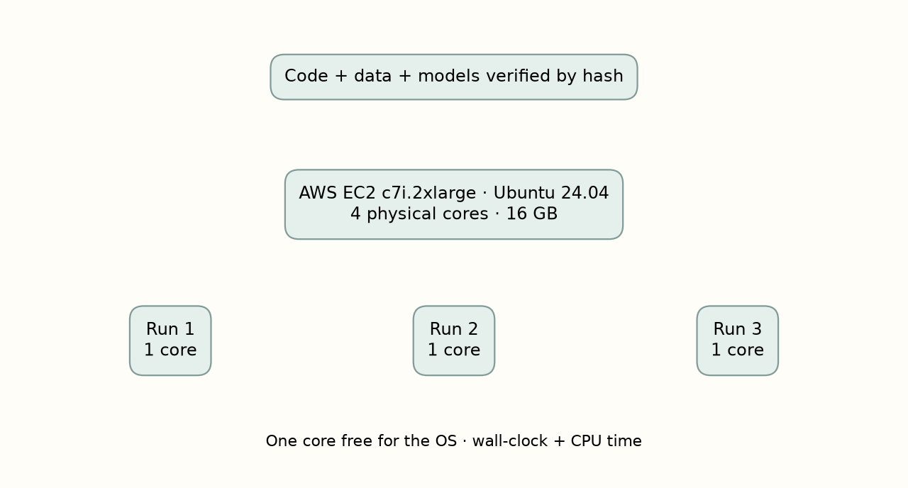
In the Python environment, I kept the research code byte-identical and checked data and models using hashes. Versions, configuration and results were recorded in manifests. Linux required resolving a shared-library collision between HiGHS and OR-Tools by changing libhighs’s SONAME identifier; the algorithm was unchanged. Before testing, a calibration of 24 runs on four validation instances checked the environment and timing.
The execution script processed all five sets with the same methods, seeds and budgets, saved logs and supported retries and resumption. It also scheduled a safety shutdown after 20 hours and another after completion and result packaging. These measures control execution; they are not an AWS cost estimate. In the second round, none of the 1,390 runs was flagged for contention, CPU time divided by wall-clock time was approximately 1, and the largest budget overrun was 0.08 seconds.
The methods, without the mystery
SCIP on the full model was the direct baseline: it receives every decision and searches for a solution that respects the constraints. Linear relaxation, or LP, temporarily permits fractional values. Its solution is not necessarily an operational network, but it provides a lower cost bound and signals about which facilities are worth examining. This information is calculated for the current instance without prior training.
The GNN represents facilities and customers as two types of nodes connected by service relationships. Exchanging information along those connections allows it to learn a score for each facility. In this experiment, that score guides search; it does not replace constraints or turn a high probability into a guarantee of a good decision. Although three checkpoints were trained, optimization testing used the checkpoint from seed 0.
Adaptive expansion starts with the highest-ranked facilities and grows the domain through 20%, 40%, 60% and 100% stages, with feasibility repairs. It is like examining a shortlist first and progressively opening the catalogue rather than throwing the rest away. It can stop early if reduced costs certify that no excluded option can improve the solution and the restricted problem has been solved to optimality. Kernel search serves a similar purpose through a core of variables and additional groups; I implemented a variant rather than every detail of the original algorithm.
CLNS releases part of a solution, keeps the rest fixed and reoptimizes only the released part. It subtracts occupied capacity and charges each opening cost only once. Its neighborhoods include cost-profile groups, boundaries between groups, customers of expensive facilities and assignments that look unfavorable according to LP. The hybrid devotes half its budget to expansion and half to CLNS. I also tested rotation, adaptive weights and learned selectors, plus memory to avoid repeating unsuccessful subproblems; these selector comparisons belong to the pilots.
What does better mean?
Final cost is not the only thing that matters. If I may need an answer at any moment, the time until a useful solution appears matters too. The primal integral summarizes that trajectory: over the budget, it averages relative distance from the best known reference, clipped between 0 and 1. Before a solution exists, it is 1. Lower is better. It is neither a percentage of logistics savings nor a direct measure of processor speed.
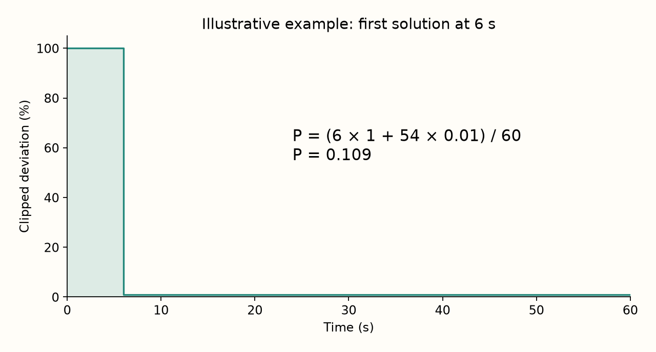
Timing included features, inference, LP, repair, model construction, solving and validation. Budgets were 60 seconds for the main synthetic and corridor cases, 120 for larger cases and Olist, and 30 for Holmberg. I averaged seeds within each instance before comparing instances. I used bootstrap intervals, paired Wilcoxon tests and Holm correction. The confirmation rule was set before repeating the test: significance at 5% in the cloud and the same direction in the local round.
The result that changed how I viewed the GNN
In everyday terms, a paired comparison tests methods on the same scenarios. Bootstrap resampling estimates uncertainty by drawing those scenarios again; Holm correction controls false positives across multiple hypotheses. A p-value alone measures neither the size of an improvement nor the probability that an explanation is true, which is why I also report magnitudes, intervals and whether the finding repeated.
On the 64 synthetic instances in the AWS round, LP expansion achieved a mean integral of 0.0326 versus 0.0611 for full SCIP: approximately 47% lower on that metric. GNN expansion reached 0.0712. Replacing only the LP ranking with the learned ranking worsened the integral by 0.0385 on average; LP won on 45 of 64 instances, with an adjusted p-value of approximately 0.005. The direction of this result repeated in both environments.
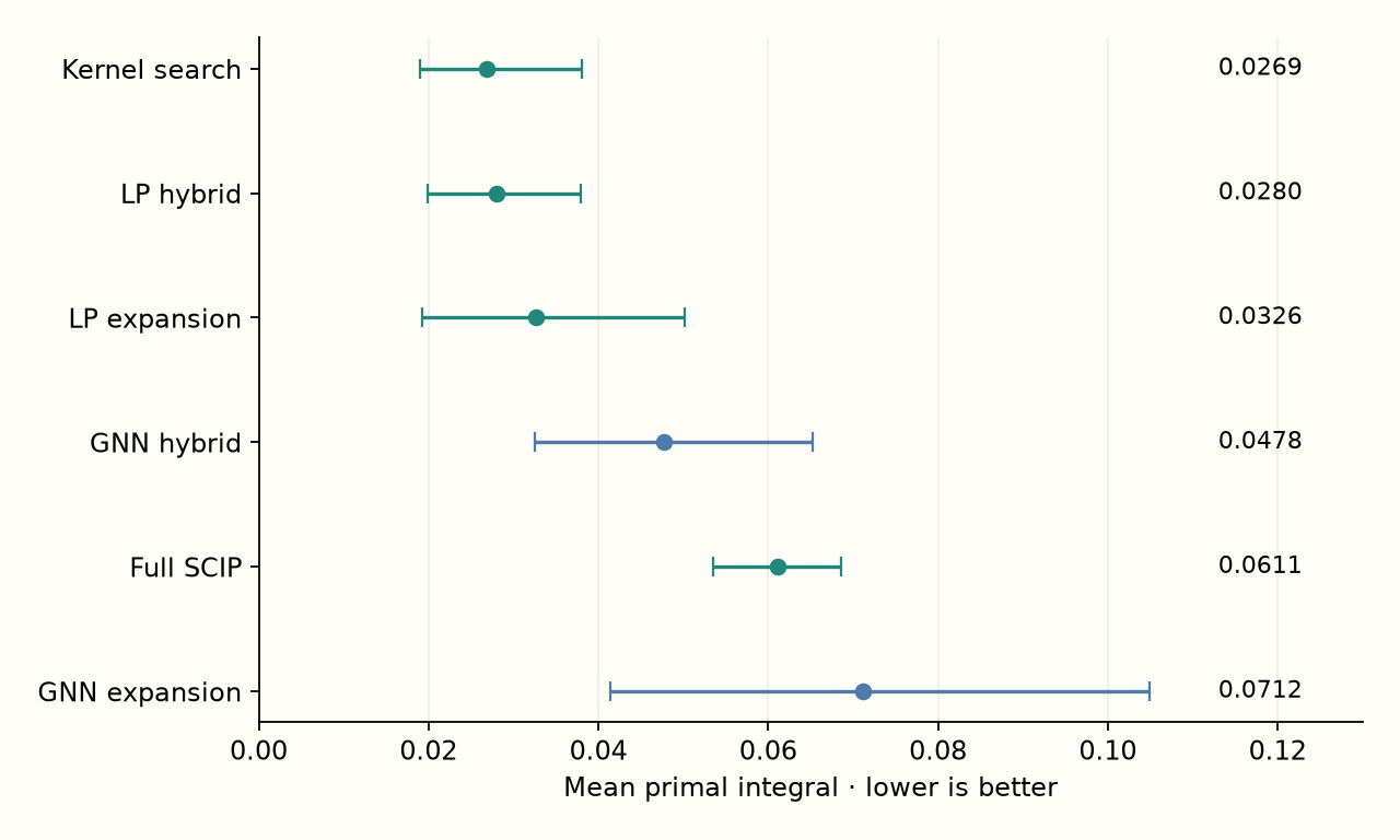
However, I did not confirm that the GNN finished with worse cost: that secondary comparison had an adjusted p-value of 0.056. Nor did I confirm a general improvement from adding CLNS to LP expansion. Kernel search had the lowest numerical integral, 0.0269, but no difference from LP expansion was established. A sorted table always has a first place; that does not make every distance between rows a robust finding.
The first sign of this problem was already visible in filtering. An AUC near 0.95 indicated good classification, yet retaining the reference solution in at least 80% of instances required keeping approximately 80% of facilities. Predicting a label well does not guarantee retaining the complete combination needed to serve all demand. Capacity and single sourcing make the whole combination matter more than each isolated score.
When size changes, the answer changes too
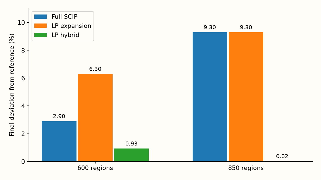
The largest Olist cases tell another part of the story. On AWS, with 600 regions, the LP hybrid finished approximately 0.93% above the best known solution, versus 2.9% for full SCIP and 6.3% for LP expansion. With 850 regions, the values were 0.02%, 9.3% and 9.3%. Here coordinated reoptimization delivered an important final improvement. These are two observations within four cases, not a guarantee for every logistics network.
Holmberg allowed another property to be checked: its known optima let me distinguish a good solution from a proof of optimality. LP expansion certified optimality before its final stage on 66 of 71 instances, with a median time of 0.4 seconds for those cases, and reached the published optimum on 67 versus 66 for the full solver. These are small instances by current standards; I did not transfer that speed claim to large cases.
Investigating why a search stalls
In the pilots, 54–58% of selected subproblems had already failed in the same local state. Memory reduced repetition to approximately 25–27%, but did not produce a conclusive quality improvement. I later repeated 256 subproblems with more time: 252 finished with proven optimality and no improvement; only four improved with 30 seconds. These diagnostics used validation instances and are exploratory. They suggest that waiting longer did not address the main obstacle in those cases.
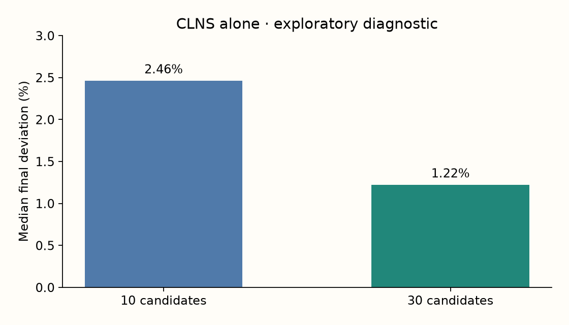
Increasing candidate facilities per customer from 10 to 30 changed standalone CLNS: median final deviation fell from 2.46% to 1.22%, improving 14 of 16 instances with an adjusted p-value of 0.002. Fewer subproblems were solved, but they had greater reach. In the hybrid, which starts from a better solution, this expansion did not show the same benefit. Replacing the groups with random groups of equal sizes also produced no significant difference: the evidence supports coordination, not established superiority of clustering.
What having no silver bullet means
The practical lesson is to define the objective before choosing the tool. Do we need a useful solution early, the lowest final cost, or proof of optimality? Then we need to identify constraints, compare against a classical alternative serving the same function and account for all runtime. When a GNN and an LP rule guide exactly the same expansion, the comparison separates the value of the mechanism from the value of learning.
The appendix also contains a result favorable to learning: a stabilized MPNN generalized across scale better than Mettu–Plaxton for uncapacitated location before adding local search. Other reconstructions, including swap filters and a neural model inside a location-routing MIP, did not clearly outperform their classical controls. These have different problems and budgets; I did not pool them into the main test or treat them as exact reproductions of the original papers.
My study does not prove a universal law of optimization. Its limits include one evaluated checkpoint, training on one size and two spatial families, predominantly synthetic data and heuristic references outside Holmberg. Both rounds repeat the same instances: they replicate measurement, not a new sample. They also do not establish that AWS is some percentage faster, because hardware, environment and references differ. Within those limits, the finding is useful: understanding the problem’s structure and measuring each component’s contribution mattered more than adding a network because of its name.
Sources and continuation
Editorial source: the manuscript “Learning versus classical guidance in search-space reduction for single-source capacitated facility location,” Tables 10–11 and Sections 5.3, 6.8 and 6.9. Charts use saved second-round results, except for the integral example, explicitly labeled illustrative. No new experiments were run to prepare this publication.