Where does Maricá need attention first? (1/3): the question and the data
Part 1 of the series on the Socioterritorial Conditions Index (ICST) of Maricá (RJ, Brazil). Why the municipal average does not help decide where to invest, how to turn ten official variables into a 0–100 index per census tract, and what to do when the data does not exist in the form you wanted.

In this article
If I told you that Maricá had 197,277 inhabitants in the 2022 Census and that 35% of households got water from the public network as their main source, what would you do with that information?
Probably nothing. Or rather: you would conclude that “Maricá lacks piped water”, which is true, but does not say where. And where is exactly the question a manager needs to answer when there is budget for a network project, a new Family Health Unit or a detailed risk mapping.
Maricá has grown a lot in recent decades, and it grew in the hardest way to serve: large, low-density subdivisions spread between the lagoons, the shoreline and the mountain slopes. Consolidated, well-served neighborhoods coexist with recent areas where the sewer network, the water network and public facilities have not yet arrived. The municipal average hides all of this.
This series explains how I built the Socioterritorial Conditions Index (ICST) of Maricá, an indicator from 0 to 100 calculated for each 2022 Census tract, using only official data and everything in Python. The work began as a paper for the UFRRJ postgraduate program in Data Analysis as a Method to Support Public Policy.
- Part 1 (this one): the question, the dimensions and the data. And the decisions I made when the data did not come ready-made.
- Part 2: the results. Maps, neighborhoods, districts and what the numbers show.
- Part 3: the priority areas, how far they can be trusted and the mystery of 35% versus 78% water coverage.
Three questions, one unit of analysis
The index was designed to answer three applied questions:
- How are socioeconomic, infrastructure, socio-environmental and service-access conditions distributed within the municipality?
- Which areas accumulate disadvantages and should be prioritized?
- How sensitive is that prioritization to the methodological choices I made?
The third question is the one most people forget. Every composite index carries choices (which variables, which weights, how to normalize), and if the ranking changes completely when you nudge them a little, it is useless for deciding anything. I come back to this in part 3.
The unit of analysis is the 2022 census tract, the smallest unit with official Census data. Maricá has 516 tracts, of which 483 have residents. The other 33 are lagoons, protected areas and unoccupied areas: they appear on the maps but receive no index. For managerial reading, results were also aggregated to the 49 neighborhoods and 4 districts defined by the City Hall.
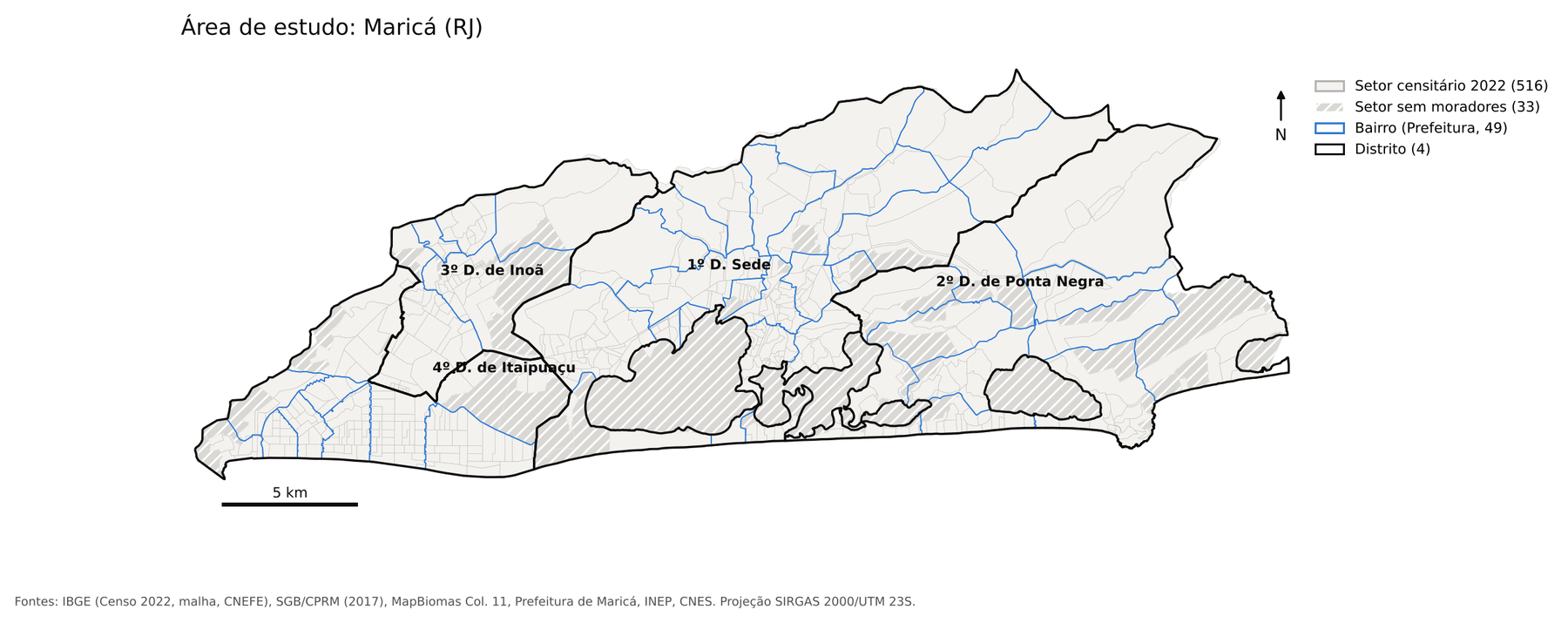
A detail that seems small and is not: when aggregating tracts into neighborhoods, I did not average percentages. I summed numerators and denominators and recalculated. Averaging percentages gives the same weight to a tract of 50 households and one of 800, and the neighborhood ends up looking better or worse than it is.
Four dimensions, ten variables
The ICST has four sub-indices. Each answers a public policy question:
| Dimension | Weight | Question | Variables |
|---|---|---|---|
| S – Socioeconomic | 0.30 | Where are income and literacy constraints concentrated? | S1 low income, S2 literacy 15+ |
| I – Infrastructure and sanitation | 0.30 | How are water, sewage and waste collection distributed? | I1 water, I2 sewage, I3 waste |
| A – Socio-environmental | 0.25 | What share of occupation is in susceptible areas and where is native vegetation being lost? | A1 flooding, A2 mass movement, A3 vegetation loss |
| P – Access to services | 0.15 | What share of households can walk to a family health unit (USF) and a public school? | P1 USF within 20 min, P2 school within 20 min |
The weights were fixed before looking at the results, as working hypotheses. Socioeconomic and infrastructure got 0.30 each because they are the most traditional dimensions and the most tied to household deprivation; access got 0.15 because it depends on location data with more uncertainty. Fixing them beforehand matters: if you choose weights after seeing the map, it is easy (and tempting) to adjust until the result “makes sense”.
Each variable was brought to a 0–100 scale using min–max normalization. For variables where a high value is bad (low income, flooding, vegetation loss), the sign is inverted. In the end, for all of them, 100 is the best situation observed in the municipality and 0 is the worst. The ICST is the weighted sum of the four sub-indices.
Where the data came from
Everything was downloaded by script, with URL, access date and SHA-256 hash recorded in a source catalog, and the original files left untouched. The main sources:
- IBGE, 2022 Census: aggregates by census tract (literacy, water, sewage, waste, income of the household head), the tract mesh and the CNEFE address registry, with 106,439 household addresses in Maricá.
- Geological Survey of Brazil (SGB/CPRM): susceptibility chart for flooding and mass movements in Maricá (2017).
- MapBiomas Collection 11: land cover and use in 2022 and 2025, at 30 m.
- Maricá City Hall: neighborhood and district boundaries and the georeferenced Family Health Units.
- INEP: schools and the 2024 School Census.
- CNES/DATASUS: health facilities, to cross-check the USFs and include those in neighboring municipalities.
- Overture Maps: road network for the walking calculation, because the municipal road base requires credentials.
- SNIS 2022 and SINISA 2024: only to compare with the Census on sanitation (spoiler from part 3: it was hard work).
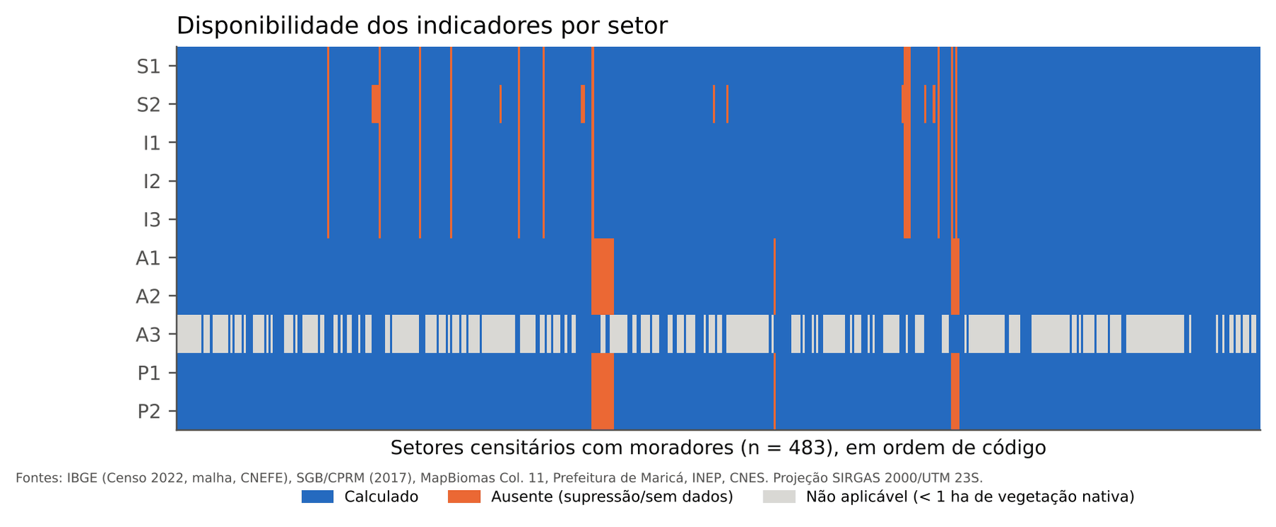
In the end, the ICST was calculated for 447 of the 483 inhabited tracts, which hold 97.5% of the population. The tracts left out are small: together they total 4,876 people.
When the data does not come the way you wanted
This is the part I would most like you to take into your own projects. The working rule was simple: do not invent data. Missing stays missing, never becomes zero or an average. But following that rule demands decisions. Four of them:
1. The 2022 Census has no income brackets by tract
The income indicator I wanted was “share of household heads earning less than 1 minimum wage”. The 2022 Census aggregate by tract has no income brackets: only the mean, variance and median of household heads’ income. The bracket table exists only at the municipal level, and the finer microdata are restricted-access.
The tempting way out would be to copy the municipal percentage to every tract. That is fabricating data. What I did was estimate the share by assuming that, within each tract, income follows a lognormal distribution (a classic hypothesis for income), with the mean and variance published by IBGE. Then I validated it three ways: the model’s implied median has a 0.96 correlation with the published median; aggregated to the 11 weighting areas, the indicator orders the areas like per-capita income in the sample; and the estimated municipal total (24.9% of heads below 1 minimum wage) is of the same order as the official distribution for the municipality.
So S1 is a modeled estimate, and I say so everywhere it appears. It works well for ranking tracts; it is not a count.
2. IBGE hides small numbers (and that is not zero)
To protect confidentiality, IBGE suppresses cells with small counts: the value appears as “X”. Treating “X” as zero would make small tracts look as if they had no water or no sewage.
Since the categories of each question add up exactly to the total number of households when nothing is suppressed, the difference between the total and what was published is the sum of the hidden cells, and each is worth at least 1. That makes it possible to compute an exact interval for the suppressed value and use its center. The lower and upper bounds went into the sensitivity analysis and did not change the ranking.
3. A household is an address, not an urban patch
To know what share of households is in a flood area or within a 20-minute walk of a USF, I need to know where the households are. The common option is to use MapBiomas’ “urbanized area” class, but it does not cover scattered subdivisions well, which is precisely Maricá’s pattern. I used CNEFE addresses: same year as the Census, address-level precision (97.6% with their own coordinates) and present in every tract with households.
4. “Not applicable” is different from “don’t know”
Native vegetation loss (A3) is a ratio: how much of the 2022 native vegetation turned into human use by 2025. In an urban tract with less than 1 hectare of native vegetation, that ratio has no basis. I marked those tracts as not applicable and recalculated the dimension using only flooding and mass movement. It was the only exception, defined before the calculation. In any other case, if a variable was missing, the tract is left without an index.
How the variables look on the map
Before putting everything into one number, it is worth looking at each variable separately. Notice how water (I1) and sewage (I2) range from 0% to 100% across tracts, while waste collection (I3) and literacy (S2) are almost universal:
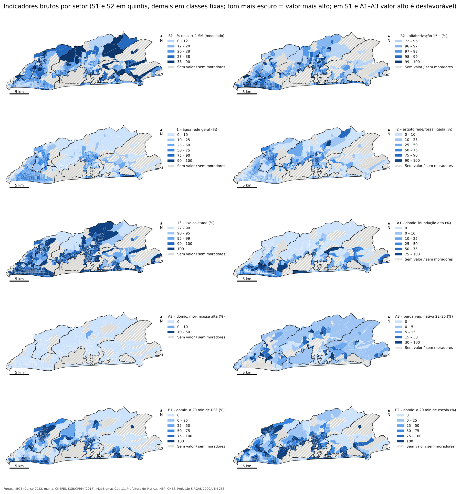
A few municipality-wide numbers to anchor us:
- Literacy at age 15 or older: median of 97.9% across tracts.
- Waste collection: 99.1% of households.
- Water from the public network as the main source: 35.2% of households.
- Sewage connected to the network: 34.7%.
- Households in high flood susceptibility: about 24.6%.
- Households within a 20-minute walk of a USF: 56.9%; of a public school with elementary education, 65.1%.
You can already suspect where inequality comes from, can’t you? It is not basic schooling or the garbage truck. It is the pipe.
In the next post, I put the ten variables together into the index and show the resulting map of Maricá: which neighborhoods and districts are doing better, which worse, and why disadvantages do not appear scattered but in patches.